Trajectory planning

Based on Chapter 4 of Robotics: Modelling, Planning and Control.

Link to the practical session on Trajectory planning

Path and trajectory planning

Path: Locus of points in joint space (or operational space) that the robot has to follow.

It is pure geometric description of motion.

Trajectory: A path on which a time law is specified in terms of velocities and/or acceleration at each point.

Trajectories must be continuous and smooth.

A single joint variable \(q(t)\) will be studied to present the approaches.

For a smooth coordination of joints, the total trajectory time is set equal to all.

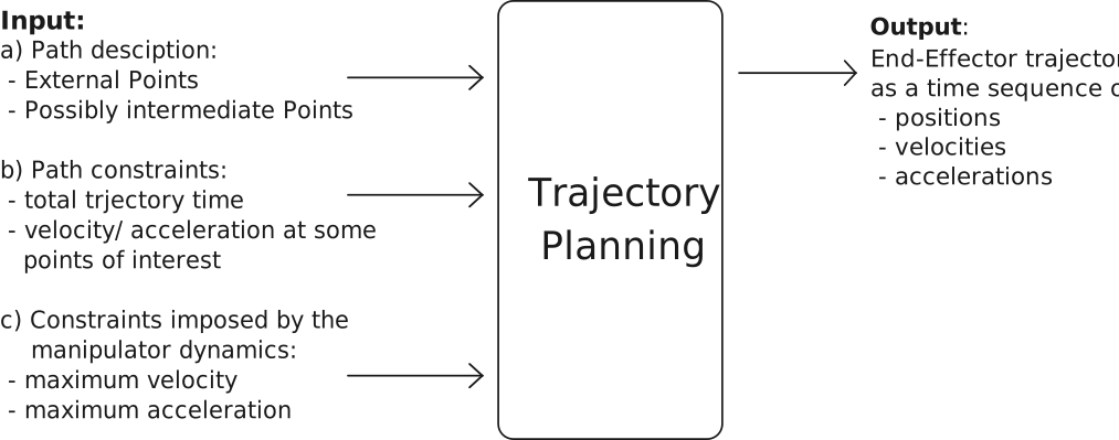
The following procedures to compute trajectories in the joint space will be first presented:

Point to point motion:

The specification includes initial and final configuration and total trajectory time.
Motion through a sequence of points:

Besides the specification of the initial and final configurations and the total trajectory time, intermediate points are specified.

Point-to-point motion

Problem: To generate a trajectory to move from \(q_i\) to \(q_f\) in a given time \(t_f\), possibly optimizing the energy dissipated by the motor \(\left(\int_{0}^{t_f} \bigl[I\,\boldsymbol{\omega}(t)\bigr]^2 \,dt\right)\).

Cubic polynomials

One solution is to determine the joint motion using cubic polynomials:

\[q(t) = a_3\,t^3 + a_2\,t^2 + a_1\,t + a_0\]

The velocity and acceleration profiles are:

\[\dot{q}(t) = 3\,a_3\,t^2 + 2\,a_2\,t + a_1\]

\[\ddot{q}(t) = 6\,a_3\,t + 2\,a_2\]

There are four coefficients: \(a_3,\,a_2,\,a_1,\,a_0\), therefore four constraints can be imposed:

\[q(0) = q_i\]

\[q(t_f) = q_f\]

\[\dot{q}(0) = \dot{q}_i \quad(\text{usually set to }0)\]

\[\dot{q}(t_f) = \dot{q}_f \quad(\text{usually set to }0)\]

Then, the following system of equation results:

\[a_0 = q_i\]

\[a_1 = \dot{q}_i\]

\[a_3\,t_f^3 + a_2\,t_f^2 + a_1\,t_f + a_0 = q_f\]

\[3\,a_3\,t_f^2 + 2\,a_2\,t_f + a_1 = \dot{q}_f\]

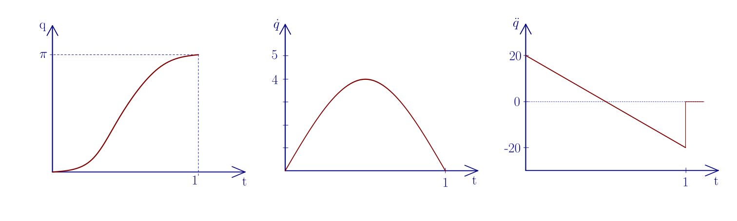
An example:

\[q_i = 0,\quad \dot{q}_i = 0,\quad q_f = \pi,\quad \dot{q}_f = 0,\quad t_f = 1\]

The solution is:

\[a_0 = 0,\quad a_1 = 0,\quad a_2 = 3\pi,\quad a_3 = -2\pi\]

Fifth-order polynomials

Alternatively, we can choose fifth-order polynomials, which will allow to fix more constraints like initial and final accelerations:

\[q(t) = a_5\,t^5 + a_4\,t^4 + a_3\,t^3 + a_2\,t^2 + a_1\,t + a_0\]

\[\dot{q}(t) = 5\,a_5\,t^4 + 4\,a_4\,t^3 + 3\,a_3\,t^2 + 2\,a_2\,t + a_1\]

\[\ddot{q}(t) = 20\,a_5\,t^3 + 12\,a_4\,t^2 + 6\,a_3\,t + 2\,a_2\]

Now there are six coefficients: \(a_5, a_4, a_3, a_2, a_1, a_0\)

And therefore six constraints can be specified: \(q(0), q(t_f), \dot{q}(0), \dot{q}(t_f), \ddot{q}(0), \ddot{q}(t_f)\)

With this option the energy dissipated by the motor is minimized.

Trapezoidal velocity profile

Another alternative frequently used in industry is a trapezoidal velocity profile:

\[\begin{split}\left\{ \begin{array}{l} \text{a constant acceleration phase}\\ \text{a cruise velocity phase}\\ \text{a constant deceleration phase} \end{array} \right.\end{split}\]

The velocity and acceleration profiles are:

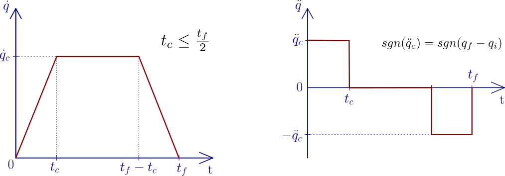
Some constraints on the velocity and acceleration must hold:

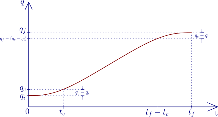
Constraint on the velocity from the values of \(q_f\), \(q_i\) and \(t_f\). The trapezoidal profile lies between the rectangular and triangular profiles, all having the same area, which is the distance traveled \(|q_f - q_i|\):

\[|\dot{q}_{c_\min}| = \frac{|q_f - q_i|}{t_f} < |\dot{q}_c| \le \frac{2\,|q_f - q_i|}{t_f} = |\dot{q}_{c_\max}|\]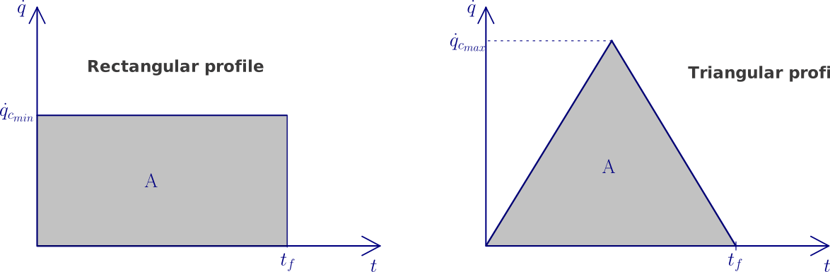
Constraint on the acceleration. It has to be greater than the one required in the triangular profile:

\[|\ddot{q}_c| \ge \frac{|\dot{q}_{c_\max}|}{t_f/2} = \frac{4\,|q_f - q_i|}{t_f}\]

Finally, the complete expression of the profile of the joint value is:

\[\begin{split}q(t) = \begin{cases} q_i + \tfrac12\,\ddot{q}_c\,t^2, & 0 \le t \le t_c\\ \\ q_c + \dot{q}_c\,(t - t_c) = \underbrace{q_i + \tfrac12\,\ddot{q}_c\,t_c^2}_{q_c} + \underbrace{\ddot{q}_c\,t_c}_{\dot{q}_c}\,(t - t_c) = q_i + \dot{q}_c\,t_c\,(t - t_c/2), & t_c < t \le t_f - t_c\\ \\ q_f - \tfrac12\,\ddot{q}_c\,(t_f - t)^2, & t_f - t_c \le t \le t_f \end{cases}\end{split}\]

Motion through a sequence of points

Problem: To generate a trajectory through a set of \(N\) points (called path points or via points), including some constraints on the velocities and/or acceleration:

\[q(t) = q_k \quad \text{for } t = t_k,\; \text{with } k = 1,\dots,N\]

\[\begin{split}\begin{cases} q_1 = q_i \\ q_N = q_f,\\ t_1 = t_i,\\ t_N = t_f \end{cases}\end{split}\]

Solution 1: Use of low-order interpolating polynomials

Usually cubic polynomials are used that allow the imposition of continuity in the velocities at the path points, i.e.,

\[q(t)\;\text{will be formed by }N-1\text{ cubic polynomials } \Pi_{k=1}^{N-1}p_k(t), \;\text{continuous and with continuous derivatives.}\]

The procedure has two steps.

Step 1: Set the velocities at the path points.

First interpolate the path points with linear segments, with slope:

\[v_k = \frac{q_k - q_{k-1}}{t_k - t_{k-1}}\]

Then the velocities at the path points are set to:

\[\begin{split}\begin{aligned} \dot{q}_k &= \begin{cases} 0, & \text{if } sgn(v_k)\neq sgn(v_{k+1}),\;k=2,\dots,N-1,\\ \\ \tfrac12\,(v_k + v_{k-1}), & \text{if } sgn(v_k)= sgn(v_{k+1}), \end{cases}\\ \dot{q}_1 &= 0\\ \dot{q}_N &= 0 \end{aligned}\end{split}\]
Step 2: Find the polynomials by solving the system of equations.

\[\begin{split}\left. \begin{eqnarray} \Pi(t_k) &=& q_k\\ \Pi(t_{k+1}) &=& q_{k+1}\\ \dot{\Pi}(t_k) &=& \dot{q}_k\\ \dot{\Pi}(t_{k+1}) &=& \dot{q}_{k+1} \end{eqnarray} \;\right\} \quad \begin{gathered} 4\text{ equations and 4 unknowns}\\ (\text{the coefficients of the cubic polynomials}) \end{gathered}\end{split}\]

Continuity of velocity is guaranteed by having fixed:

\[\dot{\Pi}_k(t_{k+1}) = \dot{\Pi}_{k+1}(t_{k+1})\]

And usually:

\[\begin{split}\begin{eqnarray} \dot{\Pi}_1(t_i) &=& \dot{q}_i = 0 \\ \dot{\Pi}_N(t_N) &=& \dot{q}_N = 0 \end{eqnarray}\end{split}\]

Solution 2: Interpolation of linear polynomials with parabolic blends

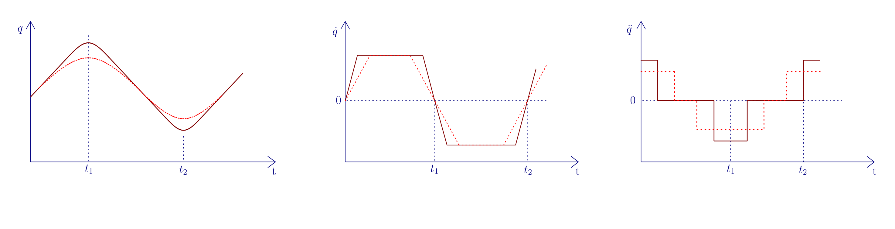
Linear interpolation is first set between path points and then, to avoid discontinuities in the first derivative, a parabolic profile (blend) around each point is permitted.

The actual trajectory does not reach the path points \(q_k\), which are called here via points.

\[\Delta t_k = \text{time distance between } q_k \text{ and } q_{k+1}\]

\[\Delta t_{k,k+1} = \text{time interval during which the interpolation is linear}\]

\[\Delta t'_k = \text{parabolic blend interval}\]

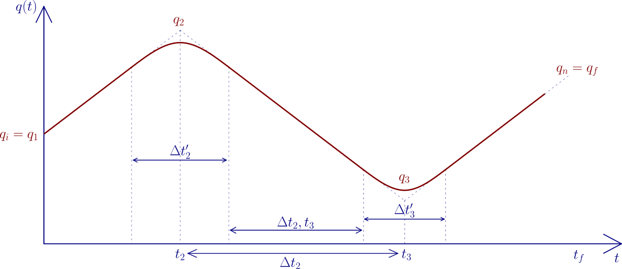
The constant velocity for the linear interval is:

\[\begin{split}\begin{eqnarray} \dot{q}_{k-1,k} &=& \frac{q_k - q_{k-1}}{\Delta t_{k-1}} \\ \dot{q}_{0,1} &=& 0 \\ \dot{q}_{N,N+1} &=& 0 \end{eqnarray}\end{split}\]
The acceleration during the parabolic blend is:

\[\ddot{q}_k = \frac{\dot{q}_{k,k+1} - \dot{q}_{k-1,k}}{\Delta t'_k}\]

Solution 3: Variant using trapezoidal profiles

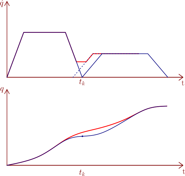
If we define trapezoidal profiles for each path between the path points, the robot will stop at them.

A variant is envisaged so as to not have zero velocity at the path points that avoid counting in starting the second segment ahead of time w.r.t. the end of the first one.

Operational-space trajectories

Sometimes the end-effector is required to follow a geometrically feasible specified path, and hence the trajectory has to be planned in the operational space since otherwise the end-effector motion is not predictable.

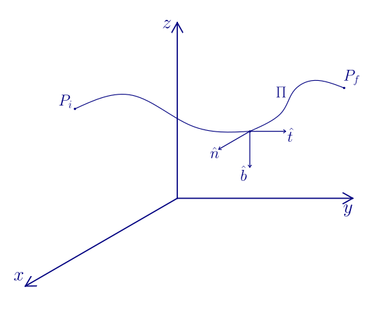
The desired trajectory has to be expressed analytically, e.g., a rectilinear or circular path.

The paths can be described in a parametric way.
The paths are sampled and the IK is performed.

Parameterization of a rectilinear path: Position

\[\begin{split}P_e(s) = P_i + \frac{s}{\|P_f - P_i\|}\,(P_f - P_i) \quad \left\{ \begin{array}{l} s \in \bigl[0,\,\|P_f - P_i\|\bigr];\, s_f = \|P_f - P_i\|\;\text{(path length)},\\ P(0) = P_i,\\ P(s_f) = P_f \end{array} \right.\end{split}\]

The parameter s is then set according to a timing law:

\[\begin{split}s = s(t) \quad \left\{ \begin{array}{l} s = 0 \quad\text{for } t = 0,\\ s = s_f \quad\text{for } t = t_f \end{array} \right.\end{split}\]

Velocity and acceleration of the end-effector along the trajectory:

\[\dot{P}_e = \frac{dP_e}{ds}\,\dot{s} = \frac{P_f - P_i}{\|P_f - P_i\|}\,\dot{s} = \hat{t}\,\dot{s}\]

Normally \(\dot{s}\) is defined with a parabolic or trapezoidal profile so that \(|\dot{P}(0)| = |\dot{P}(t_f)| = 0\)

for piece-wise linear paths, the parameter \(s\) is interpolated using any of the methods shown for \(q(t)\).

Parameterization of a rectilinear path: Orientation

a) Using Euler angles

\[\boldsymbol{\phi}_e = (\varphi, \theta, \psi),\quad \boldsymbol{\phi}_e = \boldsymbol{\phi}_i + \frac{s_i}{\|\boldsymbol{\phi}_f - \boldsymbol{\phi}_i\|} (\boldsymbol{\phi}_f - \boldsymbol{\phi}_i)\]

\[\boldsymbol{\dot{\phi}}_e = \frac{\dot{s}_i}{\|\boldsymbol{\phi}_f - \boldsymbol{\phi}_i\|} (\boldsymbol{\phi}_f - \boldsymbol{\phi}_i)\]

\[\boldsymbol{\ddot{\phi}}_e = \frac{\ddot{s}_i}{\|\boldsymbol{\phi}_f - \boldsymbol{\phi}_i\|} (\boldsymbol{\phi}_f - \boldsymbol{\phi}_i)\]

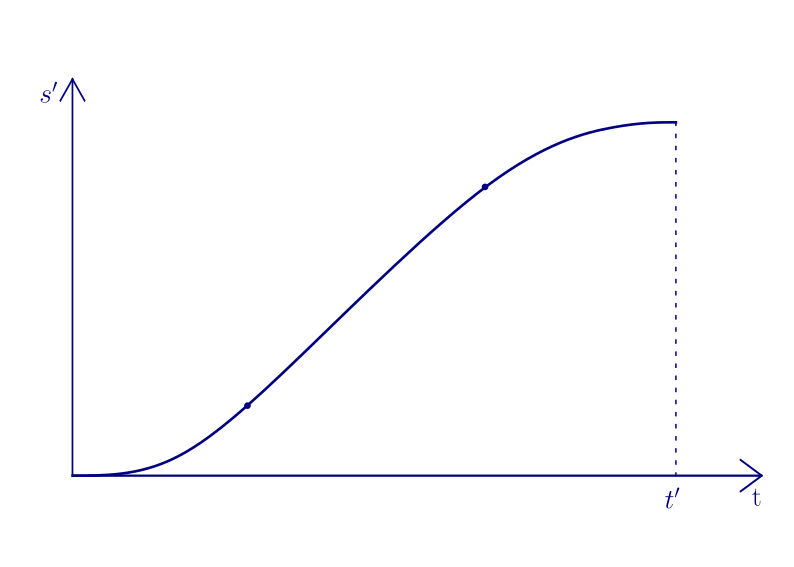
with \(s(t)\) a timing law defined with a cubic-polynomial profile or a linear profile with parabolic blends.

b) Using angle-axis:

More simple and clear interpolation since we can move from the orientation of one frame to that of another by rotating a given angle \(\theta\) about a given axis \(\boldsymbol{r}\).

\[\begin{split}\left. \begin{array}{l} R_i : \text{initial orientation w.r.t. base frame}\\ R_f : \text{final orientation w.r.t. base frame} \end{array} \right\} \quad R^i_f = \text{rotation matrix} = (\theta, \boldsymbol{r}^i)\end{split}\]

We can vary \(\theta\) as \(\theta(s)\) such that \(\theta(0)=0\) and \(\theta(s_f)=0\).
We can vary \(R^i(s)\) such that \(R^{i}(0)=I\) and \(R^{i}(s_f)=R_f^i\).

Then:

\[\begin{split}\left. \begin{aligned} R_e(s) &= R_i\,R^i(s); \,\,\,\text{results from }r\text{ and }\theta(s)\\ \omega_e(s) &= R_i\,\omega^i(s) = R_i\,\dot{\theta}(s)\,r^i,\\ \dot{\omega}_e(s) &= R_i\,\dot{\omega}^i(s) = R_i\,\ddot{\theta}(s)\,r^i \end{aligned} \!\right\} \;\text{, and }s(t)\text{ as before.}\end{split}\]