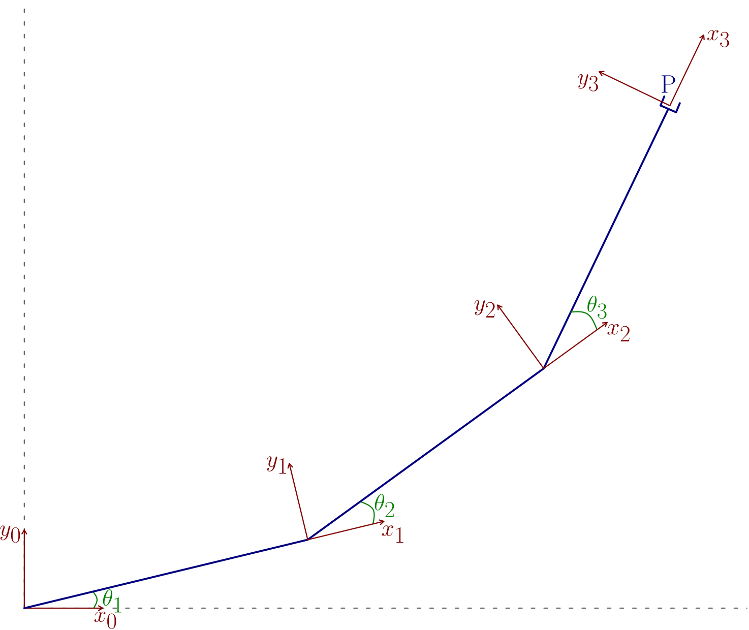
The Geometric Jacobian
a) The concept
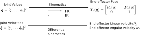
The geometric Jacobian, \(J(\boldsymbol{q})\), is a matrix that describes the differential kinematics mappings:
\[\dot{\boldsymbol P}_e = J_p(\boldsymbol{q})\,\dot{\boldsymbol q},\quad
J_p\text{ is a }(3\times n)\text{ matrix}\]
\[\omega_e = J_o(\boldsymbol{q})\,\dot{\boldsymbol q},\quad
J_o\text{ is a }(3\times n)\text{ matrix}\]
\[\begin{split}\boxed{
\boldsymbol v_e =
\begin{bmatrix}
\dot{\boldsymbol P}_e\\
\omega_e
\end{bmatrix}
=
\begin{bmatrix}
J_p(\boldsymbol{q})\\
J_o(\boldsymbol{q})
\end{bmatrix}
\dot{\boldsymbol q}
= J(\boldsymbol{q})\,\dot{\boldsymbol q}
}
\quad J\text{ is a }(6\times n)\text{ matrix}\end{split}\]
\(J(\boldsymbol{q})\) is computed with geometric techniques that determine the contribution of each joint velocity to the end-effector linear and angular velocities.
For this, the angular and linear velocities of a link will be first derived in section b, and particularized for prismatic and revolute joints in section c.
Then, section d gives the expression of the Jacobian, and section e includes some demonstration of expressions used previously in section b.
b) Link angular/linear velocities
Given Frame \(i-1\), with associated linear and angular velocities \(\boldsymbol{\dot P}_{i-1}\) and \(\boldsymbol{\omega}_{i-1}\), and given Frame \(i\), attached to Link \(i\), let’s compute its associated linear and angular velocities, \(\boldsymbol{\dot P}_i\) and \(\boldsymbol{\omega}_i\), knowing the relative linear and angular velocities, \(\boldsymbol{v}_{\,i-1,i}\) and \(\boldsymbol{\omega}_{\,i-1,i}\), produced by the velocity of joint \(i\).
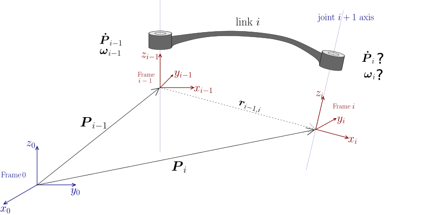
The position of the origin of Frame \(i\) is:
\[\boldsymbol{P}_i
= \boldsymbol{P}_{i-1} + R_{i-1} \boldsymbol r_{i-1,i}^{i-1}\]
Then, the linear velocity of link \(i\) is:
\[\boxed{
\boldsymbol{\dot P}_i
= \boldsymbol{\dot P}_{i-1}
+ \boldsymbol{v}_{\,i-1,i}
+ \boldsymbol{\omega}_{i-1}\times\boldsymbol{r}_{\,i-1,i}
}\]
\[\boldsymbol{v}_{\,i-1,i} \, \equiv\,\, \text{ linear velocity of the origin of frame } i \text{ w.r.t. the origin of frame } i-1.\]
\[\boldsymbol{v}_{\,i-1,i} \text{ is the contribution of the joint } i \text{ to the linear velocity of frame } i.\]
And the angular velocity of link \(i\) is:
\[\boxed{
\boldsymbol{\omega}_i
= \boldsymbol{\omega}_{i-1}
+ \boldsymbol{\omega}_{\,i-1,i}
}\]
\[\boldsymbol{\omega}_{\,i-1,i} \, \equiv\,\, \text{ angular velocity of frame } i \text{ w.r.t. frame } i-1.\]
\[\boldsymbol{\omega}_{\,i-1,i} \text{ is the contribution of the joint } i \text{ to the angular velocity of frame } i.\]
c) Prismatic/revolute joints
The relative linear and angular velocities, \(\boldsymbol{v}_{\,i-1,i}\) and \(\boldsymbol{\omega}_{\,i-1,i}\), produced by the velocity of joint \(i\), have the following expressions according to the nature of the joint:
\[\begin{split}\left.
\begin{array}{l}
\boldsymbol{v}_{\,i-1,i} = \dot{d}_i\,\,\boldsymbol{z}_{i-1}\\
\boldsymbol{\omega}_{\,i-1,i} = 0
\end{array}
\right\}
\quad\text{prismatic joints}\end{split}\]
\[\begin{split}\left.
\begin{array}{l}
\boldsymbol{v}_{\,i-1,i} = \boldsymbol{\omega}_{i-1,i}\times\boldsymbol{r}_{i-1,i}\\
\boldsymbol{\omega}_{\,i-1,i} = \dot{\theta_i}\, \boldsymbol{z}_{i-1}
\end{array}
\right\}
\quad\text{revolute joints}\end{split}\]
d) Jacobian computation
Considering the expressions of the link velocities computed in section b and the expressions of the relative linear and angular velocities computed in section c, let’s find the Jacobian by computing:
The linear velocity of the end effector, \(\dot{\boldsymbol P}_e\)
The angular velocity of the end effector, \(\boldsymbol{\omega}_e\)
Consider first the linear velocities:
\[\dot{\boldsymbol P}_e = J_p(\boldsymbol q)\,\dot{\boldsymbol q}
= \sum_{i=1}^n j_{p_i}\,\dot q_i\]
\[j_{p_i} \equiv \text{contribution of joint } i
\text{ to the linear velocity of the end-effector.}\]
If joint \(i\) is prismatic, then
\(\boldsymbol v_{\,i-1,i} = \dot d_i\,\boldsymbol z_{i-1}\), which is directly the contribution of joint \(i\) to the end-effector velocity.
\[j_{p_i}\,\dot q_i = \dot d_i\,\boldsymbol z_{i-1}
\quad\Rightarrow\quad
\boxed{
j_{p_i} = \boldsymbol z_{i-1}}\]
If joint \(i\) is revolute, then
\(\boldsymbol v_{\,i-1,i} = \boldsymbol\omega_{\,i-1,i}\times\boldsymbol r_{\,i-1,i}\). In this case, to consider the effect on the end-effector we need to use the vector \(\boldsymbol r_{\,i-1,e}\) that locates the origin of the end-effector with respect to the origin of Frame \(i-1\):
\[\boldsymbol{j}_{p_i}\,\dot q_i
= \boldsymbol\omega_{\,i-1,i}\times\boldsymbol r_{\,i-1,e}
= \dot\theta_i\,\boldsymbol z_{i-1}\times(\boldsymbol P_e - \boldsymbol P_{\,i-1})
\quad\Rightarrow\quad
\boxed{j_{p_i} = \boldsymbol z_{i-1}\times(\boldsymbol P_e - \boldsymbol P_{\,i-1})}\]
Consider now the angular velocities:
\[\boldsymbol{\omega}_e = J_{\theta}(\boldsymbol q)\,\dot{\boldsymbol q}
= \sum_{i=1}^n \boldsymbol{j}_{\theta_i}\,\dot{q}_i\]
\[\begin{split}\boldsymbol{\omega}_e = \boldsymbol{\omega}_n
= \sum_{i=1}^n \boldsymbol{\omega}_{i,i-1},
\quad\text{with}\quad
\begin{cases}
\boldsymbol{\omega}_{i-1,i} = 0 & \text{prismatic}\\
\boldsymbol{\omega}_{i-1,i} = \dot{\theta}_i\,\boldsymbol{z}_{i-1}
& \text{revolute}
\end{cases}\end{split}\]
\[\begin{split}\implies
\begin{cases}
\dot{q}_i\,\boldsymbol{j}_{\theta_i} = 0
& \text{for prismatic joints}
\quad \boxed{\boldsymbol{j}_{\theta_i} = 0},\\[6pt]
\dot{q}_i\,\boldsymbol{j}_{\theta_i} = \dot{\theta}_i\,\boldsymbol{z}_{i-1}
& \text{for revolute joints}
\quad \boxed{\boldsymbol{j}_{\theta_i} = \boldsymbol{z}_{i-1}}.
\end{cases}\end{split}\]
Finally:
\[\begin{split}\boxed{
J = \begin{bmatrix}
J_p \\[4pt]
J_\theta
\end{bmatrix}
= \begin{bmatrix}
\boldsymbol{j}_{p_1} & \dots & \boldsymbol{j}_{p_n} \\[6pt]
\boldsymbol{j}_{\theta_1} & \dots & \boldsymbol{j}_{\theta_n}
\end{bmatrix}}\end{split}\]
with
\[\begin{split}\boldsymbol{j}_{p_i} =
\begin{cases}
\boldsymbol{z}_{i-1}
& \text{for prismatic joints}\\[6pt]
\boldsymbol{z}_{i-1}\times\bigl(\boldsymbol{P}_e - \boldsymbol{P}_{\,i-1}\bigr)
& \text{for revolute joints}
\end{cases}\end{split}\]
\[\begin{split}\boldsymbol{j}_{\theta_i} =
\begin{cases}
0 & \text{for prismatic joints}\\[6pt]
\boldsymbol{z}_{i-1} & \text{for revolute joints}
\end{cases}\end{split}\]
This is a simple and systematic way to compute \(J(\boldsymbol{q})\) since vectors
\(\boldsymbol{z}_{i-1}, \boldsymbol{P_e}, \boldsymbol{P_i}\) are function of the joint configuration
\(\boldsymbol{q}\) and can be easily obtained using the forward kinematics:
\[\begin{split}a)\quad
\boldsymbol{z}_{i-1}
= R^0_{1}(q_1)\,R^1_{2}(q_2)\,\dots\,R^{\,i-2}_{\,i-1}(q_{i-1})
\begin{bmatrix}0\\0\\1\end{bmatrix}\end{split}\]
\[\begin{split}b)\quad
\tilde{P}_e
= A^0_1(q_1)\,A^1_2(q_2)\,\dots\,A^{\,n-1}_{\,n}(q_n)
\begin{bmatrix}0\\0\\0\\1\end{bmatrix}
= \begin{bmatrix}P_{e x}\\P_{e y}\\P_{e z}\\1\end{bmatrix}
= \begin{bmatrix}\boldsymbol{P}_e\\1\end{bmatrix}\end{split}\]
\[\begin{split}c)\quad
\tilde{P}_{\,i-1}
= A^0_1(q_1)\,A^1_2(q_2)\,\dots\,A^{\,i-2}_{\,i-1}(q_{i-1})
\begin{bmatrix}0\\0\\0\\1\end{bmatrix}
= \begin{bmatrix}P_{\,i-1\,x}\\P_{\,i-1\,y}\\P_{\,i-1\,z}\\1\end{bmatrix}
= \begin{bmatrix}\boldsymbol{P}_{\,i-1}\\1\end{bmatrix}\end{split}\]
e) Demonstration of b
This section gives some details on the derivation of the link velocities give in section b. It can be skiped in a first reading.
Derivative of a rotation matrix:
\[\boldsymbol{p}(t) = R(t)\,\boldsymbol{p}^1\,\,\,\, (\boldsymbol{p}^1 \text{ is a constant vector})\]
\[\boldsymbol{\dot p}(t) = \dot{R}(t)\,\boldsymbol{p}^1
= S\bigl(\omega(t)\bigr)\,R(t)\,\boldsymbol{p}^1\]
\[\omega(t) = (\omega_x,\omega_y,\omega_z)^T \equiv \text{ angular velocity of frame } R(t) \text{ w.r.t. the global frame}\]
\[\begin{split}S\bigl(\omega(t)\bigr)
= \begin{bmatrix}
0 & -\omega_z & \omega_y \\
\omega_z & 0 & -\omega_x \\
-\omega_y & \omega_x & 0
\end{bmatrix}
\quad(\text{skew-symmetric})\end{split}\]
Also, from mechanics we know that:
\[\boldsymbol{\dot p}(t) = \omega(t)\times R(t)\,\boldsymbol{p}^1\]
Therefore,
\[\boxed{\dot{R} = S(\omega)\,R = \omega\times R}\]
Also, the following holds:
\[\boxed{R\,S(\omega)\,R^T = S(R\,\omega)}\]
Linear velocity:
\[\boldsymbol{p}_i = \boldsymbol{p}_{i-1} + R_{\,i-1}\,\boldsymbol{r}^{\,i-1}_{\,i-1,i}\]
Differentiating:
\[\boldsymbol{\dot p}_i
= \boldsymbol{\dot p}_{i-1} + R_{\,i-1}\,\boldsymbol{\dot r}^{\,i-1}_{\,i-1,i}
+ \dot{R}_{\,i-1}\,\boldsymbol{r}^{\,i-1}_{\,i-1,i}\]
\[= \boldsymbol{\dot p}_{i-1} + \boldsymbol{v}_{\,i-1,i}
+ \boldsymbol{\omega}_{\,i-1}\times R_{\,i-1}\,\boldsymbol{r}^{\,i-1}_{\,i-1,i}\]
\[\boxed{\boldsymbol{\dot p}_i
= \boldsymbol{\dot p}_{i-1} + \boldsymbol{v}_{\,i-1,i}
+ \boldsymbol{\omega}_{\,i-1}\times \boldsymbol{r}^{\,i-1}_{\,i-1,i}}\]
Angular velocity:
\[R_i = R_{\,i-1}\,R^{\,i-1}_{\,i}\]
Let’s differentiate both sides of the expression:
\[\frac{d}{dt}\bigl(R_{i-1}R_{i}^{\,i-1}\bigr)
= \dot R_{i-1}\,R_{i}^{\,i-1} + R_{i-1}\,\dot R_{i}^{\,i-1}\]
\[= s\bigl(\boldsymbol\omega_{i-1}\bigr)\underbrace{\,R_{i-1}\,R_{i}^{\,i-1}}_{R_i}
+ \underbrace{\underbrace{R_{i-1}\,s\bigl(\boldsymbol\omega_{\,i-1,i}^{\,i-1}\bigr)\,R_{i}^{\,i-1}}_{R_{i-1}\,s(\boldsymbol\omega_{i-1,i}^{i-1})\,R_{i-1}^T\,R_{i-1}\,R_{i}^{\,i-1}}}_{s(R_{i-1},\boldsymbol\omega_{i-1,i})}\]
\[= s\bigl(\boldsymbol\omega_{i-1}\bigr)\,R_{i}
+ s\bigl(R_{i-1},\boldsymbol\omega_{\,i-1,i}^{\,i-1}\bigr)\,R_{i}\]
\[\frac{d}{dt}\bigl(R_i\bigr) = s\bigl(\boldsymbol\omega_i\bigr)\,R_i\]
Therefore,
\[s\bigl(\boldsymbol\omega_i,R_i\bigr)
= s\bigl(\boldsymbol\omega_{i-1}\bigr)\,R_i
+ s\bigl(R_{i-1}\boldsymbol\omega_{\,i-1,i}^{\,i-1}\bigr)\,R_i\]
which implies that:
\[\boxed{
\boldsymbol\omega_i
= \boldsymbol\omega_{i-1} + R_{i-1}\,\boldsymbol\omega_{\,i-1,i}^{\,i-1}
= \boldsymbol\omega_{i-1} + \boldsymbol\omega_{\,i-1,i}}\]
The Analytic Jacobian
Computation of \(J_A(\boldsymbol q)\)
If the end-effector pose is expressed in terms of a minimal set of parameters, i.e.,
\(X_e = \begin{bmatrix} \boldsymbol p_e \\[4pt] \boldsymbol \phi_e \end{bmatrix}\)
with \(\boldsymbol p_e = [x\; y\; z]^{T}\) and \(\boldsymbol \phi_e = [\varphi,\;\theta,\;\psi]^{T}\) (for instance, the ZYZ Euler angles), then the Jacobian can be computed analytically
by differentiating the direct kinematics.
Linear velocity:
\[\boldsymbol {\dot P}_e
= \frac{\partial \boldsymbol P_e}{\partial \boldsymbol q}\,\boldsymbol{\dot q}
= J_P(\boldsymbol q)\,\boldsymbol{\dot q}\]
Angular velocity:
\[\boldsymbol {\dot \phi}_e
= \frac{\partial \boldsymbol \phi_e}{\partial \boldsymbol q}\,\boldsymbol{\dot q}
= J_{\phi}(\boldsymbol q)\,\boldsymbol{\dot q}\]
Finally:
\[\begin{split}\boldsymbol{\dot X}_e
= \begin{bmatrix} \boldsymbol{\dot P}_e \\[4pt] \boldsymbol{\dot \phi}_e \end{bmatrix}
= \begin{bmatrix} J_P(\boldsymbol q) \\[4pt] J_{\phi}(\boldsymbol q) \end{bmatrix}\,\boldsymbol{\dot q}
= J_A(\boldsymbol q)\,\boldsymbol{\dot q}\end{split}\]
\[\boxed{
J_A(\boldsymbol q)
= \frac{\partial\,k(\boldsymbol q)}{\partial \boldsymbol q}}\]
with \(k(\,\cdot\,)\) the direct kinematics \(k(\boldsymbol q) = [\,x\; y\; z\; \varphi\;\theta\;\psi\,]^{T}\)
Relation with \(J(\boldsymbol q)\)
Considering ZYZ Euler angles:
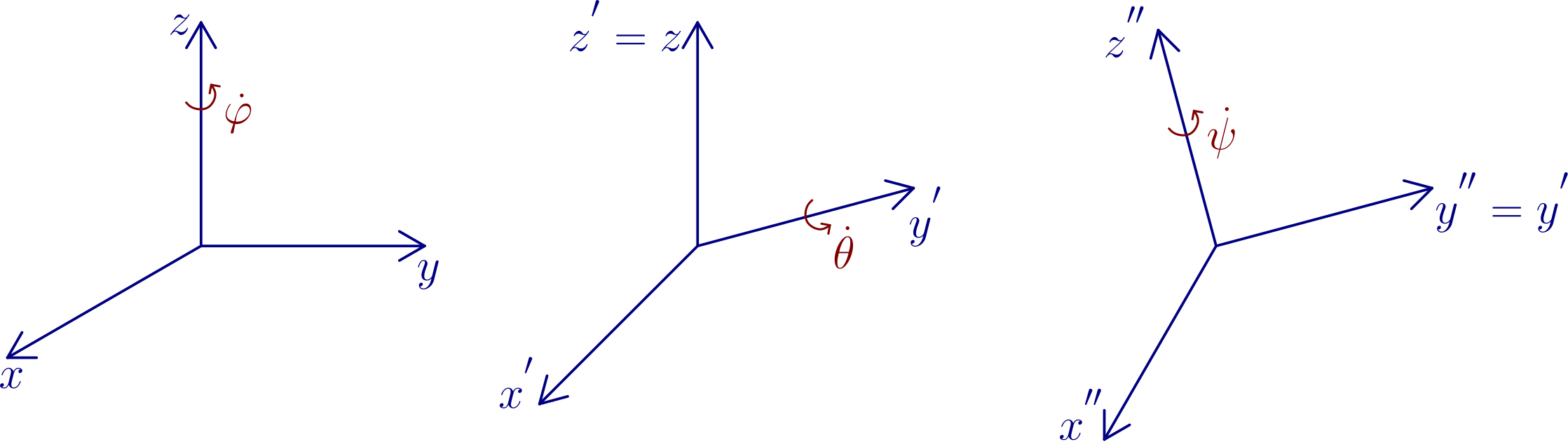
\[\begin{split}\dot\varphi \;\to\;
\begin{bmatrix}\omega_x\\\omega_y\\\omega_z\end{bmatrix}
= \dot\varphi\,\begin{bmatrix}0\\0\\1\end{bmatrix}\end{split}\]
\[\begin{split}\dot\theta \;\to\;
\begin{bmatrix}\omega_x\\\omega_y\\\omega_z\end{bmatrix}
= \dot\theta\,\begin{bmatrix}-\,s_\varphi\\c_\varphi\\0\end{bmatrix}\end{split}\]
\[\begin{split}\dot\psi \;\to\;
\begin{bmatrix}\omega_x\\\omega_y\\\omega_z\end{bmatrix}
= \dot\psi\,
\begin{bmatrix}
c_\varphi\,s_\theta\\
s_\varphi\,s_\theta\\
c_\theta
\end{bmatrix}\end{split}\]
Then:
\[\begin{split}\boldsymbol\omega_e
= \begin{bmatrix}\omega_x\\\omega_y\\\omega_z\end{bmatrix}
= \begin{bmatrix}
0 & -s_\varphi & c_\varphi\,s_\theta \\
0 & c_\varphi & s_\varphi\,s_\theta \\
1 & 0 & c\theta
\end{bmatrix}
\begin{bmatrix}\dot\varphi\\\dot\theta\\\dot\psi\end{bmatrix}
= T(\phi_e)\,\boldsymbol{\phi}_e\end{split}\]
The expression of \(T(\phi_e)\) depends on the Euler angles used:
\[\begin{split}T(\phi_e)
= \begin{bmatrix}
0 & -s_\varphi & c_\varphi\,s_\theta \\
0 & c_\varphi & s_\varphi\,s_\theta \\
1 & 0 & c\theta
\end{bmatrix} \quad \text{ when using ZYZ Euler angles}\end{split}\]
\[\begin{split}T(\phi_e)
= \begin{bmatrix}
1 & 0 & s_\theta \\
0 & c_\varphi & s_\varphi\,c_\theta \\
0 & s_\varphi & c_\varphi\,c_\theta
\end{bmatrix} \quad \text{ when using XYZ Euler angles}\end{split}\]
Finally:
\[\begin{split}\boldsymbol v_e
= \begin{bmatrix}\dot{\boldsymbol P}_e\\\boldsymbol\omega_e\end{bmatrix}
= \begin{bmatrix}
I & 0\\
0 & T(\boldsymbol\phi_e)
\end{bmatrix}
\begin{bmatrix} \boldsymbol{\dot P}_e\\\ \boldsymbol{\dot \phi}_e\end{bmatrix}
= T_{A}(\boldsymbol\phi_e)\,\boldsymbol{\dot X}_e\end{split}\]
\[\begin{split}\left.
\begin{aligned}
\boldsymbol v_e &= T_{A}(\boldsymbol\phi_e)\,\boldsymbol{\dot X}_e\\[6pt]
\boldsymbol v_e &= J(\boldsymbol q)\,\dot{\boldsymbol q} \\[6pt]
\dot x_e &= J_{A}(\boldsymbol q)\,\dot{\boldsymbol q}
\end{aligned}
\right\}
\quad
\boxed{J(\boldsymbol q) = T_{A}(\boldsymbol\phi_e)\,J_{A}(\boldsymbol q)}\end{split}\]
with:
\[\begin{split}T_{A}(\boldsymbol\phi_e)
= \begin{bmatrix}
I & 0\\
0 & T(\boldsymbol\phi_e)
\end{bmatrix}.\end{split}\]
Exercises
Compute \(J_{A}(\boldsymbol q)\) for the anthropomorphic arm
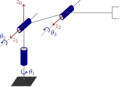
\[\begin{split}A^{0}_{3}
= \left[
\begin{array}{ccc:c}
c_{1}c_{23} & -\,c_{1}s_{23} & s_{1} & c_{1}(a_{2}c_{2} + a_{3}c_{23}) \\[6pt]
s_{1}c_{23} & -\,s_{1}s_{23} & -c_{1} & s_{1}(a_{2}c_{2} + a_{3}c_{23}) \\[6pt]
s_{23} & -c_{23} & 0 & a_{2}s_{2} + a_{3}s_{23} \\[4pt]
\hdashline
0 & 0 & 0 & 1
\end{array}
\right]\end{split}\]
Computation of the translational (linear-velocity) part:
\[\begin{split}\boldsymbol{P}_{e} =
\begin{bmatrix}
c_{1}(a_{2}c_{2} + a_{3}c_{23}\\
s_{1}(a_{2}c_{2} + a_{3}c_{23}\\
a_{2}s_{2} + a_{3}s_{23}
\end{bmatrix}\end{split}\]
\[\begin{split}\boldsymbol{\dot P}_{e}
= \frac{\partial \boldsymbol P_{e}}{\partial \boldsymbol q}\,\boldsymbol{\dot q}
= \begin{bmatrix}
\frac{\partial x}{\partial q_{1}} & \frac{\partial x}{\partial q_{2}} & \frac{\partial x}{\partial q_{3}} \\[4pt]
\frac{\partial y}{\partial q_{1}} & \frac{\partial y}{\partial q_{2}} & \frac{\partial y}{\partial q_{3}} \\[4pt]
\frac{\partial z}{\partial q_{1}} & \frac{\partial z}{\partial q_{2}} & \frac{\partial z}{\partial q_{3}}
\end{bmatrix}
\begin{bmatrix}
\dot q_{1} \\[2pt]
\dot q_{2} \\[2pt]
\dot q_{3}
\end{bmatrix}\end{split}\]
\(J_{P}(\boldsymbol q)\) is a \((3\times n)\) matrix whose components are:
\[\frac{\partial x}{\partial q_{1}} = -\,s_{1}\,\bigl(a_{2}c_{2} + a_{3}c_{23}\bigr)\]
\[\frac{\partial x}{\partial q_{2}}
= -\,c_{1}a_{2}s_{2} - c_{1}a_{3}s_{23}
= -\,c_{1}\,\bigl(a_{2}s_{2} + a_{3}s_{23}\bigr)\]
\[\frac{\partial x}{\partial q_{3}} = -\,c_{1}a_{3}s_{23}\]
\[\frac{\partial y}{\partial q_{1}} = c_{1}\,\bigl(a_{2}c_{2} + a_{3}c_{23}\bigr)\]
\[\frac{\partial y}{\partial q_{2}} = -\,s_{1}\,\bigl(a_{2}s_{2} + a_{3}s_{23}\bigr)\]
\[\frac{\partial y}{\partial q_{3}} = -\,s_{1}a_{3}s_{23}\]
\[\frac{\partial z}{\partial q_{1}} = 0\]
\[\frac{\partial z}{\partial q_{2}} = a_{2}c_{2} + a_{3}c_{23}\]
\[\frac{\partial z}{\partial q_{3}} = a_{3}c_{23}\]
\[\begin{split}J_p(\boldsymbol q) =
\begin{bmatrix}
-s_1\,(a_2 c_2 + a_3 c_{23})
& -c_1\,(a_2 s_2 + a_3 s_{23})
& -c_1\,a_3 s_{23}\\[6pt]
c_1\,(a_2 c_2 + a_3 c_{23})
& -s_1\,(a_2 s_2 + a_3 s_{23})
& -s_1\,a_3 s_{23}\\[6pt]
0
& a_2 c_2 + a_3 c_{23}
& a_3 c_{23}
\end{bmatrix}\end{split}\]
Computation of the rotationa (angular-velocity) part:
\[\begin{split}R^0_3 =
\begin{bmatrix}
c_1 c_{23} & -c_1 s_{23} & s_1\\
s_1 c_{23} & -s_1 s_{23} & -c_1\\
s_{23} & c_{23} & 0
\end{bmatrix}
=
\begin{bmatrix}
r_{11} & r_{12} & r_{13}\\
r_{21} & r_{22} & r_{23}\\
r_{31} & r_{32} & r_{33}
\end{bmatrix}\end{split}\]
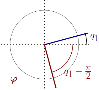
\[\varphi = \operatorname{atan2}(r_{23},\,r_{13})
= \operatorname{atan2}(-c_1,\,s_1)
= q_1 - \tfrac{\pi}{2}\]
\[\theta = \operatorname{atan2}\bigl(\sqrt{r_{13}^2 + r_{23}^2},\,r_{33}\bigr)
= \operatorname{atan2}\bigl(\sqrt{s_1^2 + c_1^2},\,0\bigr)
= \operatorname{atan2}(1,\,0)
= \tfrac{\pi}{2}\]
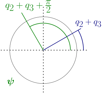
\[\psi = \operatorname{atan2}(r_{32},\,-r_{31})
= \operatorname{atan2}(c_{23},\,-s_{23})
= q_2 + q_3 + \tfrac{\pi}{2}\]
\[\begin{split}\boldsymbol{\dot{\phi}}_e
= \frac{\partial\phi_e}{\partial q}\,\boldsymbol{\dot{q}}
=
\begin{bmatrix}
\frac{\partial \varphi}{\partial q_1}
& \frac{\partial \varphi}{\partial q_2}
& \frac{\partial \varphi}{\partial q_3}\\[4pt]
\frac{\partial \theta}{\partial q_1}
& \frac{\partial \theta}{\partial q_2}
& \frac{\partial \theta}{\partial q_3}\\[4pt]
\frac{\partial \psi}{\partial q_1}
& \frac{\partial \psi}{\partial q_2}
& \frac{\partial \psi}{\partial q_3}
\end{bmatrix}
\begin{bmatrix}
\dot{q}_1\\
\dot{q}_2\\
\dot{q}_3
\end{bmatrix}
=
\begin{bmatrix}
1 & 0 & 0\\
0 & 0 & 0\\
0 & 1 & 1
\end{bmatrix}
\boldsymbol{\dot{q}}
= J_{\phi}(\boldsymbol{q})\,\boldsymbol{\dot{q}}\end{split}\]
Verification of the relation between Jacobians (assuming ZYZ Euler angles):
\[\begin{split}J(\boldsymbol{q})
= T_A(\phi)\,J_A(\boldsymbol{q})
= \begin{bmatrix}I & 0\\[4pt]0 & T(\phi)\end{bmatrix}
\,J_A(\boldsymbol{q})\Rightarrow
J_{\theta}(\boldsymbol{q}) = T(\phi)\,J_{\phi}(\boldsymbol{q})\end{split}\]
\[\begin{split}J_{\phi}(\boldsymbol{q}) = T(\phi)\,J_{\phi}(\boldsymbol{q}) =
= \begin{bmatrix}
0 & -s_{\varphi} & c_{\varphi}s_{\theta}\\[4pt]
0 & c_{\varphi} & s_{\varphi}s_{\theta}\\[4pt]
1 & 0 & c_{\theta}
\end{bmatrix}\,
\begin{bmatrix}
1 & 0 & 0\\[4pt]
0 & 0 & 0\\[4pt]
0 & 1 & 1
\end{bmatrix}
= \begin{bmatrix}
0 & c_{\varphi}s_{\theta} & c_{\varphi}s_{\theta}\\[4pt]
0 & s_{\varphi}s_{\theta} & s_{\varphi}s_{\theta}\\[4pt]
1 & c_{\theta} & c_{\theta}
\end{bmatrix}\end{split}\]
\[\begin{split}\left(
\varphi = q_1 - \tfrac{\pi}{2}
\implies
\begin{cases}
c_{\varphi} = s_1\\
s_{\varphi} = -c_1
\end{cases}\quad
;\,\,\,\theta = \tfrac{\pi}{2}
\implies
\begin{cases}
c_{\theta} = 0\\
s_{\theta} = 1
\end{cases}\right)\end{split}\]
\[\begin{split}J_{\phi}(\boldsymbol{q})
= \begin{bmatrix}
0 & s_1 & s_1\\[4pt]
0 & -c_1 & -c_1\\[4pt]
1 & 0 & 0
\end{bmatrix} ✅\end{split}\]
Jacobian of the spherical wrist
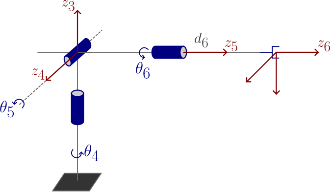
\[\begin{split}A^3_4 =
\begin{bmatrix}
c_4 & 0 & -s_4 & 0\\
s_4 & 0 & c_4 & 0\\
0 & -1 & 0 & 0\\
0 & 0 & 0 & 1
\end{bmatrix}
,\quad
A^4_5 =
\begin{bmatrix}
c_5 & 0 & s_5 & 0\\
s_5 & 0 & -c_5 & 0\\
0 & 1 & 0 & 0\\
0 & 0 & 0 & 1
\end{bmatrix}
,\quad
A^5_6 =
\begin{bmatrix}
c_6 & -s_6 & 0 & 0\\
s_6 & c_6 & 0 & 0\\
0 & 0 & 1 & d_6\\
0 & 0 & 0 & 1
\end{bmatrix}\end{split}\]
\[\begin{split}A^3_6(q) =
\begin{bmatrix}
c_4 c_5 c_6 - s_4 s_6
& -\,c_4 c_5 s_6 - s_4 c_6
& c_4 s_5
& c_4 s_5 d_6\\[6pt]
s_4 c_5 c_6 + c_4 s_6
& -\,s_4 c_5 s_6 + c_4 c_6
& s_4 s_5
& s_4 s_5 d_6\\[6pt]
-\,s_5 c_6
& s_5 s_6
& c_5
& c_5 d_6\\[6pt]
0 & 0 & 0 & 1
\end{bmatrix}\end{split}\]
Geometric Jacobian:
Since there are three revolute joints, the Jacobian is:
\[\begin{split}J(\boldsymbol{q}) =
\begin{bmatrix}
\; \boldsymbol{z}_3\times(\boldsymbol{P}_6-\boldsymbol{P}_3)
& \boldsymbol{z}_4\times(\boldsymbol{P}_6-\boldsymbol{P}_4)
& \boldsymbol{z}_5\times(\boldsymbol{P}_6-\boldsymbol{P}_5)\;\\[6pt]
\boldsymbol{z}_3 & \boldsymbol{z}_4 & \boldsymbol{z}_5
\end{bmatrix}\end{split}\]
The \(\boldsymbol{z}\) axes are:
\[\begin{split}\boldsymbol{z}_3 = \begin{bmatrix}0\\0\\1\end{bmatrix}\end{split}\]
\[\begin{split}\boldsymbol{z}_4 = R^3_4(q_4)\begin{bmatrix}0\\0\\1\end{bmatrix}
= \begin{bmatrix}
c_4 & 0 & -s_4\\
s_4 & 0 & -c_4 \\
0 & -1 & 0
\end{bmatrix} \quad
\begin{bmatrix}
0\\
0\\
1
\end{bmatrix}
= \begin{bmatrix}-s_4\\c_4\\0\end{bmatrix}\end{split}\]
\[\begin{split}\boldsymbol z_{5} = R_{4}^{3}(q_{4})\,R_{5}^{4}(q_{5})
\begin{bmatrix}0\\0\\1\end{bmatrix}
=
\begin{bmatrix}
c_{4} & 0 & -s_{4} \\
s_{4} & 0 & c_{4} \\
1 & 0 & 0
\end{bmatrix}
\begin{bmatrix}
c_{5} & 0 & s_{5} \\
s_{5} & 0 & -c_{5} \\
0 & 1 & 0
\end{bmatrix}
\begin{bmatrix}0\\0\\1\end{bmatrix}
=
\begin{bmatrix}
c_{4} & 0 & -s_{4} \\
s_{4} & 0 & c_{4} \\
0 & -1 & 0
\end{bmatrix}
\begin{bmatrix} s_{5} \\ -c_{5} \\ 0 \end{bmatrix}
=
\begin{bmatrix}
c_{4}s_{5} \\
s_{4}s_{5} \\
c_{5}
\end{bmatrix}\end{split}\]
And the origins of the reference frames are:
\[\begin{split}\tilde{ P}_{3}
= \begin{bmatrix}0\\0\\0\\1\end{bmatrix}
,\quad
\tilde{ P}_{4}
= A_{4}^{3}(q_{4}) \begin{bmatrix}0\\0\\0\\1\end{bmatrix}
= \begin{bmatrix}0\\0\\0\\1\end{bmatrix}
,\quad
\tilde{ P}_{5}
= A_{4}^{3}A_{5}^{4}\begin{bmatrix}0\\0\\0\\1\end{bmatrix}
= \begin{bmatrix}0\\0\\0\\1\end{bmatrix}\end{split}\]
\[\begin{split}\tilde{ P}_{6}
= A_{4}^{3}A_{5}^{4}A_{6}^{5}\begin{bmatrix}0\\0\\0\\1\end{bmatrix}
= A_{4}^{3}A_{5}^{4}\begin{bmatrix}0\\0\\d_{6}\\1\end{bmatrix}
= A_{4}^{3}\begin{bmatrix}s_{5}d_{6}\\-c_{5}d_{6}\\0\\1\end{bmatrix}
= \begin{bmatrix}
c_{4}s_{5}d_{6}\\
s_{4}s_{5}d_{6}\\
c_{5}d_{6}
\end{bmatrix}\end{split}\]
Then, the translational terms are:
\[\begin{split}\boldsymbol z_{3} \times \tilde{ P}_{6}
= \begin{vmatrix}
i & j & k \\
0 & 0 & 1 \\
c_{4}s_{5}d_{6} & s_{4}s_{5}d_{6} & c_{5}d_{6}
\end{vmatrix}
=
\begin{bmatrix}
-s_{4}s_{5}d_{6} \\
c_{4}s_{5}d_{6} \\
0
\end{bmatrix}\end{split}\]
\[\begin{split}\boldsymbol z_{4} \times \tilde{ P}_{6}
= \begin{vmatrix}
i & j & k \\
-s_{4} & c_{4} & 0 \\
c_{4}s_{5}d_{6} & s_{4}s_{5}d_{6} & c_{5}d_{6}
\end{vmatrix}
=
\begin{bmatrix}
c_{4}c_{5}d_{6} \\
s_{4}c_{5}d_{6} \\
-s_{5}d_{6}
\end{bmatrix}\end{split}\]
\[\begin{split}\boldsymbol z_{5} \times \tilde{ P}_{6}
= \begin{vmatrix}
i & j & k \\
c_{4}s_{5} & s_{4}s_{5} & c_{5} \\
c_{4}s_{5}d_{6} & s_{4}s_{5}d_{6} & c_{5}d_{6}
\end{vmatrix}
=
\begin{bmatrix}
0 \\ 0 \\ 0
\end{bmatrix}\end{split}\]
Finally:
\[\begin{split}J(\boldsymbol q)
=
\begin{bmatrix}
-\,s_{4}s_{5}d_{6} & c_{4}c_{5}d_{6} & 0 \\
c_{4}s_{5}d_{6} & s_{4}c_{5}d_{6} & 0 \\
0 & -\,s_{5}d_{6} & 0 \\
\hdashline
0 & -\,s_{4} & c_{4}s_{5} \\
0 & c_{4} & s_{4}s_{5} \\
1 & 0 & c_{5}
\end{bmatrix}\quad
= \begin{bmatrix}
J_{P}(\boldsymbol q) \\[4pt]
J_{\theta}(\boldsymbol q)
\end{bmatrix}\end{split}\]
Analytical Jacobian:
\[\begin{split}\boldsymbol P_{e}
= \begin{bmatrix}
c_{4}s_{5}d_{6} \\[4pt]
s_{4}s_{5}d_{6} \\[4pt]
c_{5}d_{6}
\end{bmatrix}\end{split}\]
\[\frac{\partial x}{\partial q_{4}} = -\,s_{4}s_{5}d_{6}
\quad
\frac{\partial y}{\partial q_{4}} = c_{4}s_{5}d_{6}
\quad
\frac{\partial z}{\partial q_{4}} = 0\]
\[\frac{\partial x}{\partial q_{5}} = c_{4}c_{5}d_{6}
\quad \,\,\,\,\,\,
\frac{\partial y}{\partial q_{5}} = s_{4}c_{5}d_{6}
\quad
\frac{\partial z}{\partial q_{5}} = -\,s_{5}d_{6}\]
\[\frac{\partial x}{\partial q_{6}} = 0
\quad\,\,
\frac{\partial y}{\partial q_{6}} = 0
\quad
\frac{\partial z}{\partial q_{6}} = 0\]
\[\begin{split}J_{P}(\boldsymbol q)
= \begin{bmatrix}
-\,s_{4}s_{5}d_{6} & c_{4}c_{5}d_{6} & 0 \\
c_{4}s_{5}d_{6} & s_{4}c_{5}d_{6} & 0 \\
0 & -\,s_{5}d_{6} & 0
\end{bmatrix}\end{split}\]
\[\begin{split}R^{3}_{6}
= \begin{bmatrix}
c_{4}c_{5}c_{6} - s_{4}s_{6}
& -\,c_{4}c_{5}s_{6} - s_{4}c_{6}
& c_{5}s_{5} \\[6pt]
s_{4}c_{5}c_{6} + s_{4}s_{6}
& -\,s_{4}c_{5}s_{6} + c_{4}c_{6}
& s_{4}s_{5} \\[6pt]
-\,s_{5}c_{6}
& s_{5}s_{6}
& c_{5}
\end{bmatrix}
=
\begin{bmatrix}
r_{11} & r_{12} & r_{13} \\
r_{21} & r_{22} & r_{23} \\
r_{31} & r_{32} & r_{33}
\end{bmatrix}\end{split}\]
\[\varphi
= \mathrm{atan2}\bigl(r_{23},\,r_{13}\bigr)
= \mathrm{atan2}\bigl(s_{4}s_{5},\,c_{4}s_{5}\bigr)
= \mathrm{atan2}\bigl(s_{4},\,c_{4}\bigr)
= q_{4}\]
\[\theta
= \mathrm{atan2}\Bigl(\sqrt{r_{13}^{2} + r_{23}^{2}},\,r_{33}\Bigr)
= \mathrm{atan2}\bigl(s_{5},\,c_{5}\bigr)
= q_{5}\]
\[\psi
= \mathrm{atan2}\bigl(r_{32},\,-r_{31}\bigr)
= \mathrm{atan2}\bigl(s_{5}s_{6},\,s_{5}c_{6}\bigr)
= q_{6}\]
\[\begin{split}\boldsymbol{\dot \phi}_e
= \begin{bmatrix}
\frac{\partial \varphi}{\partial q_{4}} & \frac{\partial \varphi}{\partial q_{5}} & \frac{\partial \varphi}{\partial q_{6}} \\[6pt]
\frac{\partial \theta}{\partial q_{4}} & \frac{\partial \theta}{\partial q_{5}} & \frac{\partial \theta}{\partial q_{6}} \\[6pt]
\frac{\partial \psi}{\partial q_{4}} & \frac{\partial \psi}{\partial q_{5}} & \frac{\partial \psi}{\partial q_{6}}
\end{bmatrix}
= \begin{bmatrix}
1 & 0 & 0 \\[6pt]
0 & 1 & 0 \\[6pt]
0 & 0 & 1
\end{bmatrix}\end{split}\]
Check:
\[J_{\phi}(\boldsymbol q) = T\bigl(\boldsymbol\phi_e\bigr)\,J_{A}(\boldsymbol q)\]
\[\begin{split}\mathrm{ZYZ}\;\implies\;\;T(\phi)
= \begin{bmatrix}
0 & -\,s_{\phi} & c_{\phi}\,s_{\theta} \\[6pt]
0 & \quad c_{\phi} & s_{\phi}\,s_{\theta} \\[6pt]
1 & \quad 0 & c_{\theta}
\end{bmatrix}
,\quad
J_{A}(\boldsymbol q)
= \begin{bmatrix}
1 & 0 & 0 \\[6pt]
0 & 1 & 0 \\[6pt]
0 & 0 & 1
\end{bmatrix}\end{split}\]
\[\begin{split}T(\phi)\,J_{A}(\boldsymbol q)
=
\begin{bmatrix}
0 & -\,s_{\phi} & c_{\phi}\,s_{\theta} \\[6pt]
0 & \quad c_{\phi} & s_{\phi}\,s_{\theta} \\[6pt]
1 & \quad 0 & c_{\theta}
\end{bmatrix}
\begin{bmatrix}
1 & 0 & 0 \\[6pt]
0 & 1 & 0 \\[6pt]
0 & 0 & 1
\end{bmatrix}
=
\begin{bmatrix}
0 & -\,s_{4} & c_{4}\,s_{5} \\[6pt]
0 & \quad c_{4} & s_{4}\,s_{5} \\[6pt]
1 & \quad 0 & c_{5}
\end{bmatrix}\end{split}\]
\[\begin{split}J_{\phi}(\boldsymbol q)
=
\begin{bmatrix}
0 & -\,s_{4} & c_{4}\,s_{5} \\[6pt]
0 & \quad c_{4} & s_{4}\,s_{5} \\[6pt]
1 & \quad 0 & c_{5}
\end{bmatrix} ✅\end{split}\]