Trajectory planning
Based on chapter 3 and chapter 7 of Robotics, Vision and Control by Peter Corke, and on chapter 4 of Robotics: Modelling, Planning and Control by Siciliano, Sciavicco, Villani and Oriolo.
It uses the The robotics toolbox for MATLAB.
Link to the theoretical session on Kinematics
Trajectories: Interpolation motions
The Robotics Toolbox incorporates both polynomial interpolation and trapezoidal interpolation.
Polynomial Interpolation
The trajectory between two points can be obtained by using quintic polynomials (![t\in[0,T]](../_images/math/98ce1e69b8688fcb31e2694ca9672348d8a20ff1.png) ):
):
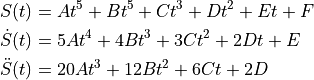
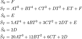
with the following specifications:
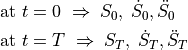
The trajectory is found by solving the following system of equations (six equations and six unknowns):
The Robotics Toolbox has the function tpoly that allows to interpolate between  and
and  considering
  , for a given time interval t, e.g. t=[0:0.02:2]. If not specified, the velocities are defaulted to zero.
>> t=[0:0.02:2];
>> [q,qd,qdd] = tpoly(0,1,t);
>> plot(t,[q,qd,qdd])
Trapezoidal Interpolation
The function lspb does this interpolation considering, by default, acceleration/cruise/decelarion phases with equal duration:
>> t=[0:0.02:2];
>> [q,qd,qdd] = lspb(0,1,t);
>> figure
>> plot(t,[q,qd,qdd])
Joint-space trajectories
The function jtraj uses the polynomial interpolation implemented in tpoly to interpolate the motion between two robot configurations (however the function mtraj can be configured to work with either tpoly or lspb).
>> mdl_puma560
>> Ti = transl(0.4,0.2,0)*trotx(pi)
>> Tf = transl(0.4,-0.2,0)*trotx(pi/2)
>> qi = p560.ikine6s(Ti)
>> qf = p560.ikine6s(Tf)
>> t=[0:0.02:2];
>> [q,qd,qdd] = jtraj(qi,qf,t)
>> qplot(t,q)
Alternatively, this can be done by using the method jtraj from the SerialLink class, and animated using the method plot:
>> q = p560.jtraj(Ti,Tf,t)
>> figure
>> p560.plot(q)
Let’s visualize how the position and orientation of the tool frame varies along the path:
>> T = p560.fkine(q)
>> p = transl(T)
>> plot(t,p)
>> xlabel('time')
>> ylabel('xyz')
>> figure
>> plot(t,tr2rpy(T))
>> xlabel('time');
>> ylabel('rpy')
In the xy-plane we can see that the position does not vary in a rectilinear way:
>> figure
>> plot(p(:,1), p(:,2))
>> xlabel('x')
>> ylabel('y')
The Robotics Toolbox also offers a Simulink file to visualize this example:
>> sl_jspace
>>> EXERCISE
 Use sl_jspace to reproduce the previous example. Repeat for different initial and  goal configurations.
Other Simulink blocks provided by the Toolbox can be found by calling:
>> roblocks
Cartesian-space trajectories
When straight-line motions in Cartesian space are required, we can use the ctraj function:
>> Ts = ctraj(Ti,Tf,length(t))
>> ps = transl(Ts)
>> plot(t,ps)
>> xlabel('time')
>> ylabel('xyz')
>> figure
>> plot(t,tr2rpy(Ts))
>> xlabel('time');
>> ylabel('rpy')
In the xy-plane we can see that now the position varies in a rectilinear way:
>> figure
>> plot(ps(:,1), ps(:,2))
>> xlabel('x')
>> ylabel('y')
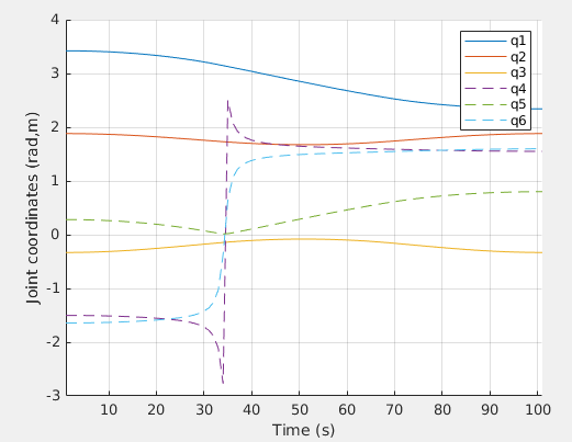
The corresponding trajectory in the joint space is:
>> qs = p560.ikine6s(Ts)
>> figure
>> qplot(qs)
>> figure
>> p560.plot(qs)
There are only slight differences in the joint trajectory with respect to the previous one, but these make the motion in Cartesian space be rectilinear.
>>> EXERCISE
 Repeat for:
  - Ti = transl(0.5, 0.3,0.44)*troty(pi/2)
  - Tf = transl(0.5, -0.3,0.44)*troty(pi/2)
 What happens at the rate of change of joints *q4* and *q6*?