Singularities and Redundancy
Based on Sections 3.3 and 3.4 of Robotics: Modelling, Planning and Control.
Link to the practical session on Differential Kinematics
Singularities
a) Definition and classification
The differential kinematics mapping given by the Jacobian, depends on \(\boldsymbol q\):
Those configurations \(\boldsymbol q\) where \(J(\boldsymbol q)\) is rank deficient are called kinematic singularities, and have the following features:
At singularities the mobility of the structure is reduced (it is not possible to impose an arbitrary end-effector velocity),
At singularities the IK may have infinite solutions,
In the neighborhood of a singularity, small velocities in the operational space may produce large velocities in the joint space.
Singularities can classified into:
Boundary singularities: Occur when the robot is either outstretched/retracted. It can be avoided if the manipulator remains inside the reachable workspace.
Internal singularities: Occur inside the reachable workspace and are generally caused by the alignment of two or more axes of motion. These may become a serious problem if paths have been planned in operational space.
Example:
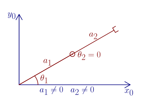
Consider the two-link planar manipulator, whose Jacobian is:
The determinant of the Jacobian is \(\det(J) = a_{1}a_{2}s_{2}\), which vanishes for \(s_{2}=0\), i.e. there are two singularities that correspond to the boundary of the workspace:
\(\theta_{2}=0\), corresponding to the arm completely outstretched, as in the figure below
\(\theta_{2}=\pi\), corresponding to the arm completely retracted
For these values of \(\theta_{2}\), the two columns of \(J\) become parallel and the rank becomes 1, so that the components of \(\boldsymbol v_e\) are not independent.
b) Decoupling
For a manipulator with a spherical wrist, the problem of singularities can be decoupled into two separate problems:
Arm singularities
Wrist singularities
Considering a 6-joint manipulator, the Jacobian can be partitioned into four \(3 \times 3\) blocks:
For the spherical wrist \(q_{4}\), \(q_{5}\), and \(q_{6}\) are revolute joints. Therefore:
In a spherical wrist all joint axes intersect at a point \(\boldsymbol P_{3} = \boldsymbol P_{4} = \boldsymbol P_{5}\). If we choose to place \(\boldsymbol P_{e}\) also at this point, then \(J_{12} = [0\;0\;0]\), i.e., \(J\) becomes a block-lower diagonal matrix whose determinant is:
i.e. a singularity decoupling has been achieved:
c) Wrist singularity
Consider the Jacobian of the spherical wrist:
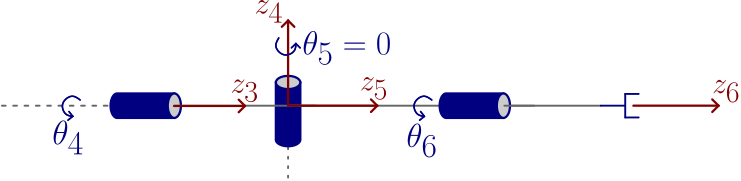
There is a singularity whenever \(\boldsymbol z_{3}\), \(\boldsymbol z_{4}\), and \(\boldsymbol z_{5}\) are linearly dependent.
Taking a look at the kinematic structure we see that this occurs when \(\boldsymbol z_{3}\) and \(\boldsymbol z_{5}\) are aligned, i.e., whenever \(\theta_{5}=0\) (like in the figure below) or \(\theta_{5}=\pi\).
We can see that in this situation:
Rotations of equal magnitude and opposite sign in \(\theta_{4}\) and \(\theta_{6}\) do not produce any change in the orientation of the end-effector (at singularities the IK may have infinite solutions).
No rotation is allowed about the axis \(\boldsymbol z_{4}\times\boldsymbol z_{5}\) (at singularities the mobility of the structure is reduced).
This is an internal singularity, we can find it in configurations within the reachable workspace.
d) Arm singularities
They depend on the arm kinematic structure. Let’s consider here an anthropomorphic arm (with \(a_{2},a_{3}\neq 0\)), whose Jacobian is:
The determinant is \(\det(J) = -\,a_{2}\,a_{3}\,s_{3}\,\bigl(a_{2}c_{2} + a_{3}c_{23}\bigr)\), which vanishes when:
Case \(s_{3}=0\) (boundary singularity):
Occurs whenever \(\theta_{3}=0\) or \(\theta_{3}=\pi\), i.e. whenever the arm is retracted or outstretched.
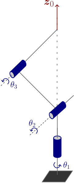
Case \(a_{2}c_{2} + a_{3}c_{23} = 0\) (internal singularity of the shoulder):
Occurs whenever the wrist point is aligned with \(\boldsymbol z_{0}\) (i.e., \(P_{x}=P_{y}=0\)), as shown in the figure below.
Note that:
A rotation around \(\theta_{1}\) doesn’t produce any change in the position of the end-effector (at singularities the IK may have infinite solutions).
No motion is allowed along the \(\boldsymbol z_{1}\) direction (at singularities the mobility of the structure is reduced).
Note
Arm singularities are well defined in operational space.
They can be easily avoided when planning in this space; this doesn’t happen with the wrist singularities.
Redundancy
a) Definitions
Consider:
n: number of DOF of the manipulator
m: number of operational space variables
r: number of operational space variables necessary to specify a task \((r \le m)\)
When \(n > r\) the manipulator is said to be kinematically redundant:
If, moreover \(n > m\) then the manipulator is said to be intrinsically redundant, since it is kinematically redundant for any task. As an example, a 7-DOF manipulator is intrinsically redundant for tasks in SE(3).
Otherwise, i.e. when \(n \not> m\) the manipulator is said to be functionally redundant. As an example, a planar manipulator with three links is functionally redundant if the task is only concerned with \(x-y\) positions.
b) The range space and the null space of J
Redundancy analysis is done using differential kinematics, which is now reformulated according to the task:
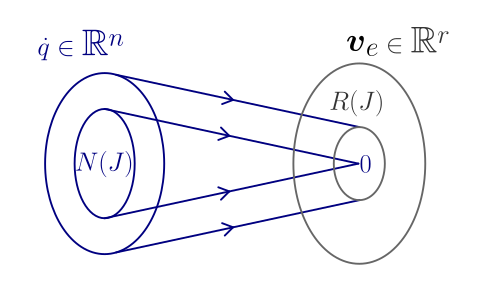
The following subspaces can be characterized in this differential kinematics mapping:
R(J) = Range space of J
It is a subspace in \(\mathbb{R}^r\) composed of all the end-effector velocities that can be generated by the joint velocities in the given manipulator configuration.
N(J) = Null space of J
It is a subspace in \(\mathbb{R}^n\) composed of all the joint velocities that do not produce any end-effector velocity in the given manipulator configuration.
When the Jacobian is full rank then:
And the following relation holds:
This relation also holds when the Jacobian is not full rank. Then, at a singularity:
The Jacobian loses rank and the dimension of the range space decreases (\(\;\Rightarrow\;\) the mobility of the structure is reduced).
According to the above expression, the dimension of the null space increases accordingly (\(\;\Rightarrow\;\) the IK may have infinite solutions).
c) Exploiting Redundancy
If \(\boldsymbol{\dot q}^{*}\) is a velocity that produces a given end-effector velocity \(\boldsymbol v_{e}^{*}\), then the composition of \(\boldsymbol{\dot q}^{*}\) with any joint velocity in the null space will produce the same \(\boldsymbol v_{e}^{*}\).
Consider a matrix \(P\) that projects any joint velocity onto the null space, i.e. the range space of \(P\) is the null space of \(J\):
Then, if we define a velocity \(\boldsymbol{\dot q}\) such that:
The following results:
Note
We can choose arbitrary joint velocities \(\boldsymbol{\dot q}_{0}\) to move the joints without moving the end-effector, allowing reconfiguration to move to more dexterous configurations.
Inverse differential kinematics
a) The problem
The inverse differential kinematics determines the joint velocities required to move the end-effector at a given operational space velocity:
Obviously the above expression is valid only if \(J\) is square.
When \(J\) is not a square matrix, this is solved by the following optimization problem:
Given \(J\) and \(\boldsymbol v_e\), find \(\boldsymbol{\dot q}\) such that \(\boldsymbol v_e = J(\boldsymbol q)\boldsymbol {\dot q}\) is satisfied and a quadratic cost function of the velocities is minimized, e.g.:
\[g(\boldsymbol{\dot q}) = \tfrac12\,\boldsymbol{\dot q}^{T}\,W\,\boldsymbol{\dot q}\]where \(W\) is a \((n\times n)\) positive semidefinite matrix of weights.
Using Lagrange multipliers the following solution to the optimization problem is obtained:
If we consider the weighting matrix to be the identity, then:
This is the right pseudo-inverse (Moore-Penrose): \(J^{+} = J^{T}(J\,J^{T})^{-1}\).
Therefore, the inverse differential kinematics when \(J\) is not a square matrix is:
b) How to specify \(g(\boldsymbol{\dot q})\) to exploit redundancy
The function to be minimized in the above stated optimization problem can be modified to include other constraints, like:
This leads to a solution as close as possible to \(\boldsymbol{\dot q}_{0}\), where \(\boldsymbol{\dot q}_{0}\) will be selected to satisfy some desired features, as detailed below.
Now the solution obtained using Lagrange multipliers is:
This is one of the matrices \(P\) that project to the null space.
Then, considering \(\boldsymbol v_e = 0\), internal motions can be described by \((I_{n} - J^{+}J)\,\dot{\boldsymbol q}_{0}\) to reconfigure the manipulator without changing the end-effector pose.
c) Alternatives for \(\boldsymbol{\dot q}_0\)
Let us consider \(\omega(\boldsymbol q)\) as a secondary objective function of the joint variables.
Then, the following expression for \(\boldsymbol{\dot q}_0\) pursues the satisfaction of this objective:
Typical objective functions are:
a) Manipulability measure:
\[\omega(\boldsymbol q) = \sqrt{\det\!\bigl(J(\boldsymbol q)\,J^{T}(\boldsymbol q)\bigr)}\]Manipulability vanishes at singularities; then by using this objective function, solutions will be found far away from singularities.
b) Distance from mechanical joints:
\[\boldsymbol{\omega}(\boldsymbol q) = -\,\frac{1}{2n}\sum_{i=1}^{n} \left(\frac{q_{i}-q_{id}} {q_{iM}-q_{im}}\right)^{2},\]where \(q_{im}\), \(\,\,\,\,q_{iM}\) and \(\,\,\,\,q_{id}\) are the min, max and mid joint values.
c) Distance to obstacles:
\[\boldsymbol{\omega}(\boldsymbol q) = \min_{\boldsymbol P,\boldsymbol \theta}\;\|\boldsymbol P(\boldsymbol q)\;-\;\boldsymbol \theta\|,\]where \(\boldsymbol \theta\) ie the position vector of an obstacle and \(\,\,\,\,\boldsymbol P\) a generic point on the structure.