Statics and manipulability

Based on Sections 3.8 and 3.9 of Robotics: Modelling, Planning and Control.

Link to the practical session on Differential Kinematics

Statics

Let:

\[\begin{split} \begin{aligned} &r \text{ be dimension of the operational space of interest}\\ &n \text{ be number of joints}\\ &\boldsymbol \tau \text{ be the } (n\times1)\;\text{vector of joint torques}\\ &\boldsymbol \gamma_{e} \text{ be the } (r\times1)\;\text{vector of end-effector forces} \end{aligned}\end{split}\]

Then, the relation between \(\boldsymbol \tau\) and \(\boldsymbol \gamma_{e}\) can be derived from the principle of virtual work and is:

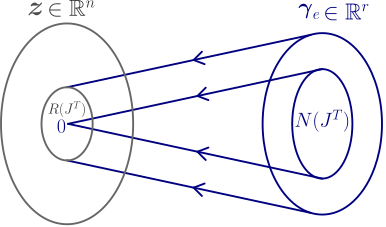
\[\boxed{ \boldsymbol \tau = J^{T}(\boldsymbol q)\,\boldsymbol \gamma_{e}}\]

Range space of \(J^{T},\, R(J^T)\): A subspace in \(\mathbb{R}^{n}\) of the joint torques that can balance the end-effector forces in a given manipulator posture.
Null space of \(J^{T}, \,N(J^T)\): A subspace in \(\mathbb{R}^{r}\) of the end-effector forces that do not require any balancing torques in the given manipulator posture.

There exists a kino-static duality:

\[\begin{split}\begin{cases} \boldsymbol v_{e} = J(\boldsymbol q)\,\boldsymbol{\dot q},\\[6pt] \boldsymbol \tau = J^{T}(\boldsymbol q)\,\boldsymbol \gamma_{e} \end{cases}\end{split}\]

Manipulability

\[\begin{split}\left. \begin{aligned} &\text{Differential kinematic equation:}\\ &\boldsymbol v_{e} = J(\boldsymbol q)\,\dot{\boldsymbol q}\\ &\text{Statics equation:}\\ &\boldsymbol \tau = J^{T}(\boldsymbol q)\,\boldsymbol F_{e} \end{aligned} \right\}\quad \text{Allow the definition of indices for the evaluation of manipulator performance.}\end{split}\]

The performance indices will be useful for:

The mechanical design of manipulators.
The determination of manipulator postures to execute a given task.

a) The velocity manipulability ellipsoid

Characterizes the set of end-effector velocities that can be obtained for a given set of joint velocities.

Consider joint velocities of unit norm:

\[\boldsymbol{\dot q}^{T}.\boldsymbol{\dot q} = 1\]

These velocities describe points on the surface of a sphere in the joint velocity space.

Then, the velocities at the end-effector generated by them are:

\[\bigl(J^{-1}\,\boldsymbol v_{e}\bigr)^{T}\,\bigl(J^{-1}\,\boldsymbol v_{e}\bigr) = 1\]

\[\boldsymbol v_{e}^{T}\,J^{-T}\,J^{-1}\,\boldsymbol v_{e} = 1\]

\[\boldsymbol v_{e}^{T}\,\bigl(J\,J^{T}\bigr)^{-1}\,\boldsymbol v_{e} = 1\]

This equation represents the points on the surface of an ellipsoid in the end-effector velocity space (see Appendix. General Equation of an Ellipsoid):

The direction of the ellipsoid axes is determined by the eigenvectors of \(J\,J^{T}\).
The dimension of each axis is given by the singular values of \(J\), \(\sigma_{i} = \sqrt{\lambda_{i}}\), where \(\lambda_{i}\) are the eigenvalues of \(J\,J^{T}\).

For redundant manipulators, the same result is obtained by using the right pseudo-inverse \(J^{+} = J^{T}\,(J\,J^{T})^{-1}\).

Note

In the direction of a major axis \(\implies\) the end-effector can move at large velocities.
In the direction of a minor axis \(\implies\) the end-effector can move only at small velocities.

Therefore, the velocity manipulability ellipsoid characterizes the manipulation ability of the kinematic structure (at this configuration) in terms of velocities.

The volume of the ellipsoid as a measure to evaluate the manipulation ability

The volume is:

\[\omega(\boldsymbol q) = \sqrt{\det\!\bigl(J(\boldsymbol q)\,J^{T}(\boldsymbol q)\bigr)}\]

If \(r = n\), this reduces to:

\[\omega(\boldsymbol q) = \bigl\lvert\det\bigl(J(\boldsymbol q)\bigr)\bigr\rvert\]

As an example consider the two-link planar manipulator:

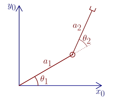
The Jacobian and its determinat are:

\[\begin{split}J = \begin{bmatrix} -\,a_{1}s_{1}-a_{2}s_{12} & -\,a_{2}s_{12} \\[6pt] a_{1}c_{1}+a_{2}c_{12} & \quad a_{2}c_{12} \end{bmatrix}\end{split}\]

\[\det(J) = a_{1}\,a_{2}\,s_{2}\]

Then, the manipulability measure is:

\[\omega(\boldsymbol q) = \bigl\lvert\det(J)\bigr\rvert = a_{1}\,a_{2}\,\lvert s_{2}\rvert\]

Note that:

The manipulability is maximum for \(\theta_{2} = \pm \tfrac{\pi}{2}\).
For a given constant reach \((a_{1} + a_{2})\), the maximum manipulability is achieved when \(a_{1} = a_{2}\) (the human arm has \(a_{1}\approx a_{2}\), and when performing dexterous tasks like writing, selects a posture with \(\theta_{2}\approx \tfrac{\pi}{2}\)).
\(\omega = 0\) when in a singular configuration:

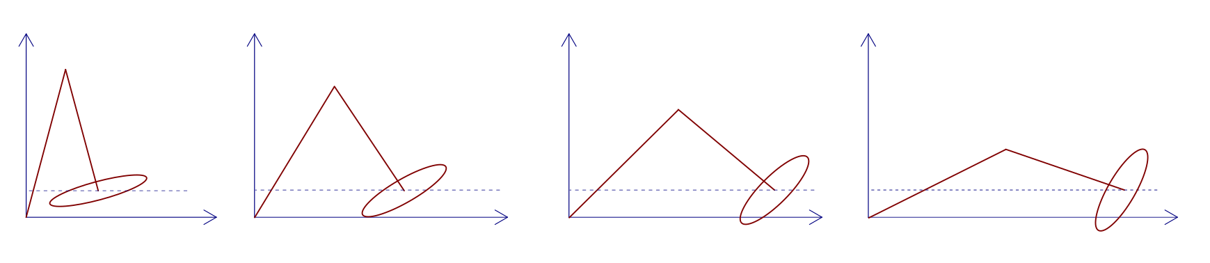
\[\begin{split}\begin{cases} \theta_{2} = 0\quad(\text{outstretched})\\[6pt] \theta_{2} = \pi\quad(\text{retracted}) \end{cases}\end{split}\]

Comments:

The value of \(\omega\) gives information on the manipulability, but the absolute value of \(\omega\) does not give us an idea of the closeness to the singularities (e.g., consider the value of \(\omega\) for an arm with \(a_{1}=a_{2}=1\text{ m}\), and another with \(a_{1}=a_{2}=1\text{ cm}\)!).
In this structure, \(\lvert s_{2}\rvert\) would be a more meaningful measure.
Not always possible to find such a meaningful measure.

The Ratio between higher and lower singular values of \(J\) as a measure to evaluate the manipulation ability

Being \(\lambda_{i}\) the eigenvalues of \(J\,J^{T}\), consider the following ratio:

\[\frac{\sigma_{r}}{\sigma_{i}} = \frac{\sqrt{\lambda_{r}}}{\sqrt{\lambda_{i}}},\]

This ratio is the inverse of the condition number of the matrix \(J\).

This ratio:

Gives the distance to the singularity.
Gives an idea about the eccentricity of the ellipsoid.

Drawback:

Computational complexity: It is practically impossible to compute in symbolic form as a function of the joint configurations.

b) The force manipulability ellipsoid

Characterizes the set of end-effector forces that can be exerted for a given set of joint torques.

Consider joint torques of unit norm:

\[\boldsymbol\tau^{T}\,\boldsymbol\tau = 1\]

Then, the end-effector forces generated by them satisfy:

\[\boldsymbol \gamma_{e}^{T}\,\bigl(J(\boldsymbol q)\,J^{T}(\boldsymbol q)\bigr)\,\boldsymbol \gamma_{e} = 1\]

The core of this quadratic form is the inverse of the previous one:

The axes of the force manipulability ellipsoid are the same as those of the velocity manipulability ellipsoid.
The dimensions along the respective axes are in inverse proportion.

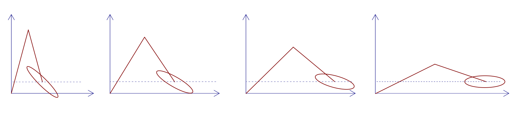
\[\begin{split} \implies \quad \begin{cases} \text{good velocity manipulability} \;\Longleftrightarrow\; \text{poor force manipulability}\\[4pt] \text{poor velocity manipulability} \;\Longleftrightarrow\; \text{good force manipulability} \end{cases}\end{split}\]

For operational spaces of dimension greater than 3, we usually separate:

linear velocity (force)
angular velocity (moment)

c) Application to given tasks

Actuation task: The task of actuating a velocity requires a large dimension of the ellipsoid along the actuating axis. The same applies for force.
Control task: The task of controlling a velocity requires a small dimension of the ellipsoid along the controlling axis so as to gain good sensitivity to errors. The same applies for force.

Due to duality: An optimal direction to actuate a velocity is also an optimal direction to control a force.

Example: A writing task needs:

Fine control of the normal force to the table.
Fine control of the velocity along the writing direction on the table.

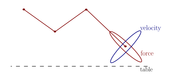
\[\begin{split} \implies \quad \begin{cases} \text{Velocity ellipsoid: small dimension }\parallel\text{ to the table, large dimension }\perp\text{ to the table}\\[4pt] \text{Force ellipsoid: small dimension }\perp\text{ to the table, large dimension }\parallel\text{ to the table} \end{cases}\end{split}\]

A 3-link planar arm mimicking the human arm.

Appendix. General Equation of an Ellipsoid

A general ellipsoid (possibly rotated and shifted) in n-dimensional space is written as a quadratic form:

\[(\mathbf{x} - \mathbf{x}_0)^T \, A \, (\mathbf{x} - \mathbf{x}_0) = 1\]

where:

\(\mathbf{x} = [x_1, x_2, \ldots, x_n]^T\) is a point in n-dimensional space,
\(\mathbf{x}_0= [x_{0,1}, x_{0,2}, \ldots, x_{0,n}]^T\) is the center of the ellipsoid, and
\(A \in \mathbb{R}^{n \times n}\) is a symmetric positive-definite matrix that encodes the shape and orientation of the ellipsoid.

Since \(A\) is symmetric positive-definite, it admits an orthogonal eigen-decomposition:

\[A = Q \Lambda Q^{T},\]

where \(Q\) is an orthogonal matrix and \(\Lambda = \operatorname{diag}(\lambda_1,\lambda_2,\ldots,\lambda_n)\) with \(\lambda_i > 0\).

By introducing the rotated coordinates \(\mathbf{y} = Q^{T}(\mathbf{x} - \mathbf{x}_0)\), the general ellipsoid quadratic form becomes:

\[\begin{split}(\mathbf{x} - \mathbf{x}_0)^T A (\mathbf{x} - \mathbf{x}_0) = 1 \\[6pt] (\mathbf{x} - \mathbf{x}_0)^T Q \Lambda Q^{T} (\mathbf{x} - \mathbf{x}_0) = 1 \\[6pt] \mathbf{y}^T \Lambda \mathbf{y} = 1 \\[6pt] \begin{bmatrix} y_1 & y_2 & \cdots & y_n \end{bmatrix} \begin{bmatrix} \lambda_1 & 0 & \cdots & 0 \\ 0 & \lambda_2 & \cdots & 0 \\ \vdots & \vdots & \ddots & \vdots \\ 0 & 0 & \cdots & \lambda_n \end{bmatrix} \begin{bmatrix} y_1 \\ y_2 \\ \vdots \\ y_n \end{bmatrix} = 1 \\[6pt] \lambda_1 y_1^2 + \lambda_2 y_2^2 + \cdots + \lambda_n y_n^2 = 1.\end{split}\]

Then, considering the semi-axes lengths:

\[a_i = \frac{1}{\sqrt{\lambda_i}}, \quad i = 1,\ldots,n,\]

the standard form of an ellipsoid in n-dimensional space (in rotated coordinates) results:

\[\frac{y_1^2}{a_1^2} + \frac{y_2^2}{a_2^2} + \cdots + \frac{y_n^2}{a_n^2} = 1, \qquad \mathbf{y} = Q^{T}(\mathbf{x} - \mathbf{x}_0).\]

Note that:

The columns of \(Q\) are the principal directions of the ellipsoid.
Each column vector corresponds to the orientation of one semi-axis in the original coordinate system.

Note

The quadratic form may also appear written using the inverse of the shape matrix, namely

\[\mathbf{x}^T A^{-1} \mathbf{x} = 1.\]

In this case, if

\[A = Q \Lambda Q^T,\]

the semi-axis lengths of the ellipsoid are given by

\[a_i = \sqrt{\lambda_i}, \quad i = 1,\ldots,n,\]

and the principal directions are again given by the columns of \(Q\).