Direct Kinematics

Based on Section 2.9 of Robotics: Modelling, Planning and Control.

Link to the practical session on Forward Kinematics

Definition

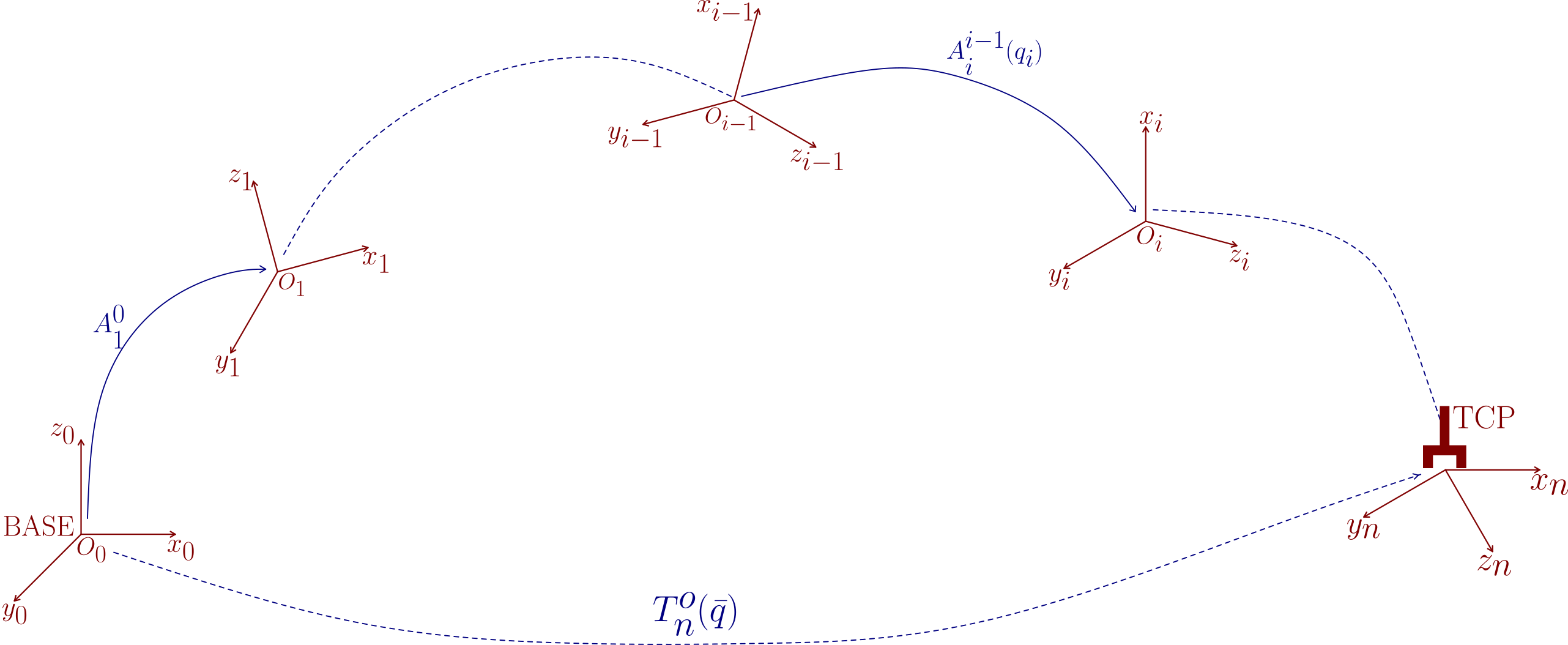
Consider a kinematic chain with:

  • \(n\) joints \(q_1, \dots, q_n\)

  • \(n+1\) links \(0, \dots, n\)

../../_images/kinematics1.1.svg

And consider the pose of the End-Effector (EE) with respect to the Base represented with a minimum number of coordinates i.e:

\[\begin{split}\boldsymbol{x_e} = \begin{bmatrix} \boldsymbol{p_e} \\ \boldsymbol{\phi_e} \end{bmatrix}; \quad \text{where} \quad \begin{cases} \boldsymbol{p_e} \text{ is the position of the EE frame} \\ \boldsymbol{\phi_e} \text{ are the Euler angles representing the orientation of the EE frame} \end{cases}\end{split}\]

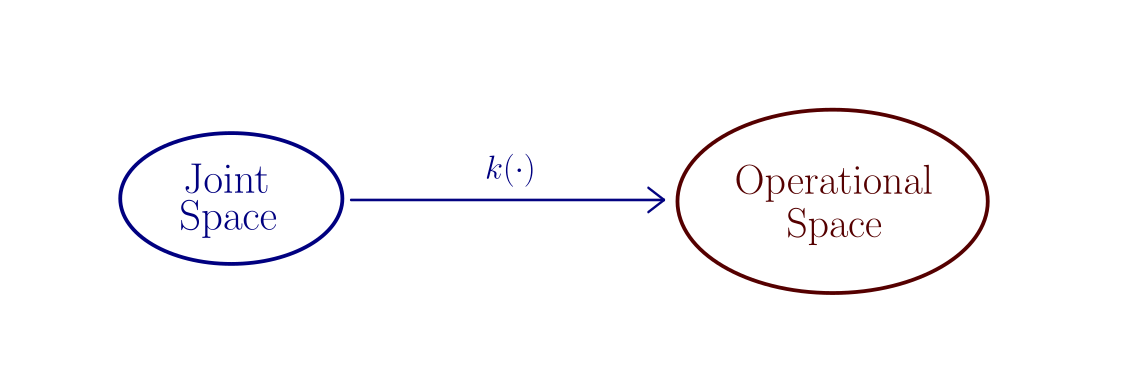
The Direct Kinematics (or Forward Kinematics) maps the joint values to the pose of the End-Effector, i.e., it maps the joint space with the operational space:

\[\boldsymbol{x_e} = k(\boldsymbol{q}), \quad \text{where} \quad \boldsymbol{q} = [q_1, \cdots, q_n]^T\]
../../_images/kinematics.1.16.svg

Two concepts arise from the relation between the joint space with the operational space:

  • Workspaces:
    • Reachable workspace: region that can be attained by the EE with at-least one orientation.

    • Dexterous workspace: region that can be attained by the EE with different orientations.

    Workspaces depend on the kinematic structure and joint limits.

  • Redundancy: There is kinematic redundancy when there are more joints than the number of variables necessary to describe the task. Redundancy provides dexterity and versatility to the motions of the manipulator.

    • A industrial manipulator (\(n=6\)) is kinematically redundant when performing a welding task on a plane (\(m=2\)).

    • The human arm (\(n=7\)) is intrinsically redundant, i.e. kinematically redundant for any task in the space (\(m=6\)).

Direct Kinematics Computation

Considering the End-Effector coincident with link \(n\), and the Base with link 0, the Direct Kinematics is:

\[T_{n}^{0}(\boldsymbol{q})=A_{1}^0(q_1)A_{2}^1(q_2).........A_{n}^{n-1}(q_{n})\]

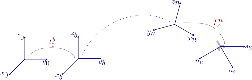
If the base is not located at link 0 and the End-Effector (TCP) is not located at link \(n\), then two fixed transforms, \(T_{b}^0\) and \(T_{e}^n\), have to be added:

\[T_{e}^{b}(\boldsymbol{q})=T_{0}^{b}T_{n}^{0}(\boldsymbol{q})T_{e}^{n}\]
../../_images/kinematics1.2.svg

The following nomenclature is sometimes used for the End-Effector frame, that assumes that it is a parallel griper:

  • \(a_e\): approach direction

  • \(s_e\): in the sliding plane of the jaws

  • \(n_e\): chosen such that (n,s,a) is right-handed

Example 2: Spherical arm

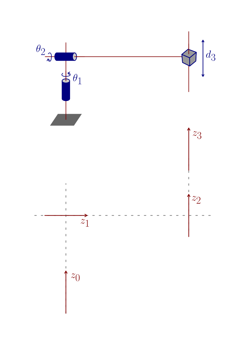
../../_images/kinematics1.5.svg

DH parameters

This manipulator has two revolute joints and a prismatic joint. The joint variables are \((\theta_1,\theta_2,d_3)\).

Follow these steps to determine the DH parameters:

  1. Set \(z\)-axis along the joint axis, made \(z_3\) arbitrarily coincident with \(z_2\) (joint 3 is prismatic).

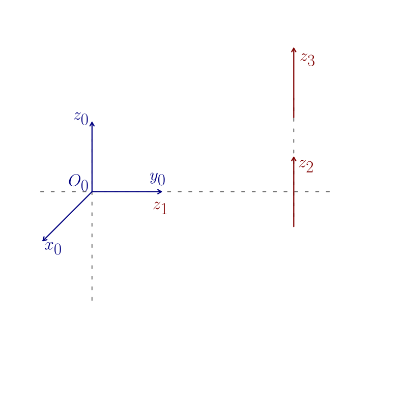
  2. Frame 0:

  • Choose \(O_0\) at the intersection of \(z_0\) and \(z_1\), to make \(d_1 = 0\).

  • Choose \(x_0\) arbitrarily.

  • Choose \(y_0\) to be right-handed.

../../_images/kinematics1.6.svg
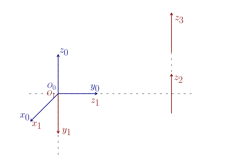
  1. Frame 1. The common normal between \(z_1\) and \(z_0\) does not exist, so:

  • Locate \(O_1\) at the intersection of \(z_1\) and \(z_0\) \(\Rightarrow a_1 = 0\).

  • Choose \(x_1\) arbitrarily. The choice done \(\Rightarrow \alpha_1 = -\frac{\pi}{2}\) (rotation about \(x_1\) to bring \(z_0\) to \(z_1\))

  • Choose \(y_1\) to be right-handed.

../../_images/kinematics1.7.svg
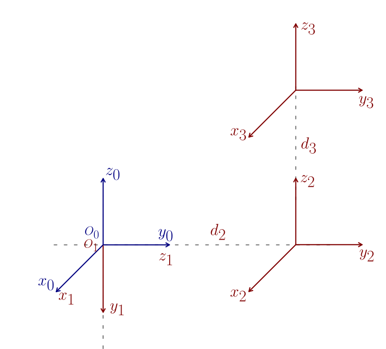
  1. Frame 2. The common normal between \(z_2\) and \(z_1\) does not exist, so:

  • Locate \(O_2\) at the intersection of \(z_2\) and \(z_1\) \(\Rightarrow a_2 = 0\).

  • Choose \(x_2\) arbitrarily- The choice done \(\Rightarrow \alpha_2 = \frac{\pi}{2}\) (rotation about \(x_2\) to bring \(z_1\) to \(z_2\)).

  • Choose \(y_2\) to be right-handed.

../../_images/kinematics1.8.svg
  1. Frame 3. There is no common normal between \(z_2\) and \(z_3\).

  • \(z_3\) has already been arbitrarily chosen (joint 3 is prismatic) coincident with \(z_2 \Rightarrow a_3 = 0, \alpha_3 = 0\).

  • Choose \(x_3\) arbitrarily.

  • Choose \(y_3\) to be right-handed.

../../_images/kinematics1.9.svg

The DH parameters are:

\[\begin{split}\begin{array}{|c|c|c|c|c|} \text{Link} & a_i & \alpha_i & d_i & \theta_i \\ \hline 1 & 0 & -\frac{\pi}{2} & 0 & \theta_1 \\ 2 & 0 & \frac{\pi}{2} & d_2 & \theta_2 \\ 3 & 0 & 0 & d_3 & 0 \\ \end{array}\end{split}\]

Homogeneous transformation between consecutive links

The homogeneous transformations are:

\[\begin{split}A_1^0 = \begin{bmatrix} c_1 & 0 & -s_1 & 0 \\ s_1 & 0 & c_1 & 0 \\ 0 & -1 & 0 & 0 \\ 0 & 0 & 0 & 1 \\ \end{bmatrix} \quad A_2^1 = \begin{bmatrix} c_2 & 0 & s_2 & 0 \\ s_2 & 0 & -c_2 & 0 \\ 0 & 1 & 0 & d_2 \\ 0 & 0 & 0 & 1 \\ \end{bmatrix} \quad A_3^2 = \begin{bmatrix} 1 & 0 & 0 & 0 \\ 0 & 1 & 0 & 0 \\ 0 & 0 & 1 & d_3 \\ 0 & 0 & 0 & 1 \\ \end{bmatrix}\end{split}\]

Direct Kinematics

\[\begin{split}T_3^0(q) = A_1^0 A_2^1 A_3^2 = \begin{bmatrix} c_1 c_2 & -s_1 & c_1 s_2 & c_1 s_2 d_3 - s_1 d_2 \\ s_1 c_2 & c_1 & s_1 s_2 & s_1 s_2 d_3 + c_1 d_2 \\ -s_2 & 0 & c_2 & c_2 d_3 \\ 0 & 0 & 0 & 1 \\ \end{bmatrix}\end{split}\]

In this case \(T_e^3 = I_3\), i.e. \((x_3, y_3, z_3) \equiv (n_e, s_e, a_e)\)

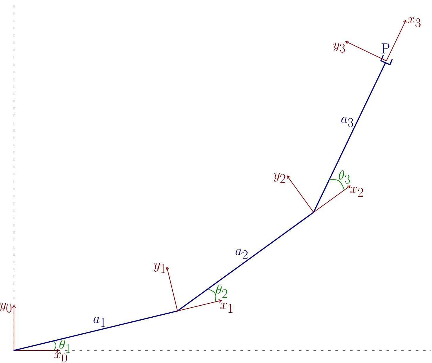
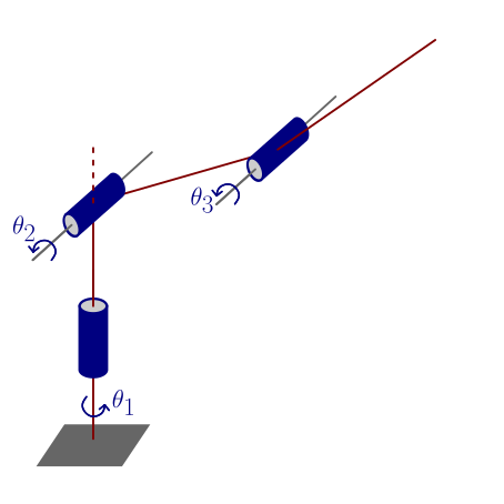
Example 3: Anthropomorphic arm

../../_images/kinematics1.10.svg ../../_images/kinematics1.12.svg

DH parameters

\[\begin{split}\begin{array}{|c|c|c|c|} & a_i & \alpha_i & d_i & \theta_i \\ \hline 1 & 0 & \frac{\pi}{2} & 0 & \theta_1 \\ 2 & a_2 & 0 & 0 & \theta_2 \\ 3 & a_3 & 0 & 0 & \theta_3 \\ \end{array}\end{split}\]

Homogeneous transformation between consecutive links

\[\begin{split}A_1^0(\theta_1) = \begin{bmatrix} c_1 & 0 & s_1 & 0 \\ s_1 & 0 & -c_1 & 0 \\ 0 & 1 & 0 & 0 \\ 0 & 0 & 0 & 1 \end{bmatrix} \qquad A_i^{i-1}(\theta_i) = \begin{bmatrix} c_i & -s_i & 0 & a_i c_i \\ s_i & c_i & 0 & a_i s_i \\ 0 & 0 & 1 & 0 \\ 0 & 0 & 0 & 1 \end{bmatrix} \quad \Rightarrow \text{like planar Manipulator}\end{split}\]

Direct Kinematics

\[\begin{split}T_3^0 = A_1^0 A_2^1 A_3^2 = \begin{bmatrix} c_1 c_{23} & -c_1 s_{23} & s_1 & c_1 (a_2 c_2 + a_3 c_{23}) \\ s_1 c_{13} & -s_1 s_{23} & -c_1 & s_1 (a_2 c_2 + a_3 c_{23}) \\ s_{23} & c_{23} & 0 & a_2 s_2 + a_3 s_{23} \\ 0 & 0 & 0 & 1 \end{bmatrix}\end{split}\]
\[\begin{split}T_e^3 = \begin{bmatrix} 0 & 0 & 1 & 0 \\ 0 & 1 & 0 & 0 \\ -1 & 0 & 0 & 0 \\ 0 & 0 & 0 & 1 \end{bmatrix} \qquad \Rightarrow \text{Maxes the end effector to have the approach along the } z_e \text{ axis.}\end{split}\]

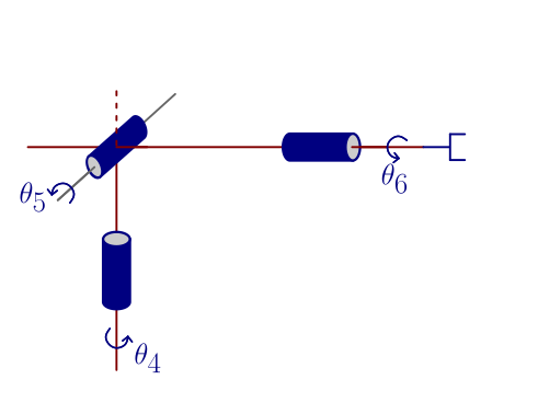
Example 4: Spherical wrist

../../_images/kinematics1.13.svg ../../_images/kinematics1.15.svg

DH parameters

All axis intersect at a single point.

\[\begin{split}\begin{array}{|c|c|c|c|} & a_i & \alpha_i & d_i & \theta_i \\ \hline 4 & 0 & -\frac{\pi}{2} & 0 & \theta_4 \\ 5 & 0 & \frac{\pi}{2} & 0 & \theta_5 \\ 6 & 0 & 0 & d_6 & \theta_6 \\ \end{array}\end{split}\]

Homogeneous transformation between consecutive links

\[\begin{split}A_4^3 = \begin{bmatrix} c_4 & 0 & -s_4 & 0 \\ s_4 & 0 & c_4 & 0 \\ 0 & -1 & 0 & 0 \\ 0 & 0 & 0 & 1 \end{bmatrix}, \quad A_5^4 = \begin{bmatrix} c_5 & 0 & s_5 & 0 \\ s_5 & 0 & -c_5 & 0 \\ 0 & 1 & 0 & 0 \\ 0 & 0 & 0 & 1 \end{bmatrix}, \quad A_6^5 = \begin{bmatrix} c_6 & -s_6 & 0 & 0 \\ s_6 & c_6 & 0 & 0 \\ 0 & 0 & 1 & d_6 \\ 0 & 0 & 0 & 1 \end{bmatrix}\end{split}\]

Direct Kinematics

\[\begin{split}T_6^4 (q) = \begin{bmatrix} c_4 c_5 c_6 - s_4 s_6 & -c_4 c_5 s_6 - s_4 c_6 & c_4 s_5 & c_4 s_5 d_6 \\ s_4 c_5 c_6 + c_4 s_6 & -s_4 c_5 s_6 + c_4 c_6 & s_4 s_5 & s_4 s_5 d_6 \\ -s_5 c_6 & s_5 s_6 & c_5 & c_5 d_6 \\ 0 & 0 & 0 & 1 \end{bmatrix}\end{split}\]

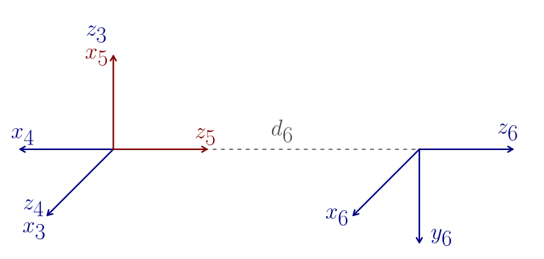
Note: That the rotation matrix \(R_6^3\) extracted from \(T_6^3\) coincides with the rotation matrix of Euler angles \(ZYZ\), i.e. the \(\theta_4, \theta_5, \theta_6\) correspond to the \(ZYZ\) Euler angles \(\varphi, \;\theta, \; \psi\) w.r.t. the reference frame \(O_3 - x_3\, y_3\, z_3\).

Finally, the frame \(6\) corresponds to an end-effector frame, i.e. the \(z_6\) is an approach direction. \((x_6\, y_6\, z_6) \equiv (n_e, s_e, a_e)\).