Inverse kinematics algorithms
Based on Sections 3.5 and 3.7 of Robotics: Modelling, Planning and Control.
The idea
We want to find joint values \(\boldsymbol{q}'\) such that the end-effector pose is \(\boldsymbol{x}_d\)
For a given configuration \(\boldsymbol{q}\) (\(\boldsymbol{q}\neq\boldsymbol{q}'\)), the end-effector pose is \(\boldsymbol{x}_e\)
The operational space error is then: \(\boldsymbol{e} = \boldsymbol{x}_d - \boldsymbol{x}_e\)
\(\Rightarrow\) Design an algorithm that keeps changing \(\boldsymbol{q}\) iteratively in such a way that the error tends asymptotically to zero, i.e., has a negative time derivative, and therefore we end with \(\boldsymbol{x}_e = \boldsymbol{x}_d\):
The analytical Jacobian (\(J_A\)) is used because we assume a minimal representation of the pose \(\boldsymbol{x}_e = (x,\;y,\;z,\;\varphi,\;\theta,\;\psi)^T\)
Jacobian pseudo-inverse method
If \(\;\;\;\boxed{\boldsymbol{\dot{q}} = J_A^{-1}(\boldsymbol{q})\,(\boldsymbol{\dot{x}}_d + k\,\boldsymbol{e})}\;\;\;\) is chosen, then the error has the following linear dynamics:
The convergence to zero of this error depends on the eigenvalues of \(k\); the larger they are, the faster the convergence. Upper bounds on these values exist since this will be implemented in discrete time (the bounds depend on the sampling time).
The algorithm can be illustrated as a control scheme:
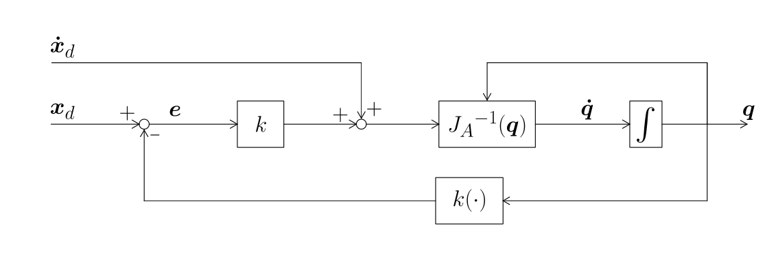
Usually \(\boldsymbol{\dot x}_d = 0\), then steady state error is null since we have integration in the loop.
For redundant manipulators the pseudo-inverse has to be used.
Jacobian transpose method
An alternative exists that does not require the inversion of \(J\).
It does not rely on the linearization of the error dynamics and therefore the Lyapunov direct method is used to ensure the asymptotic stability.
Let us define the functional \(v(\boldsymbol{e})\) as:
Differentiating:
If we choose \(\boxed{\dot{\boldsymbol{q}} = -\,J_A^T(\boldsymbol{q})\,k\,\boldsymbol{e}}\) this leads to:
If we consider the case where \(\boldsymbol{\dot x}_d = 0\) (constant reference), then \(\dot{v}<0\) is satisfied if \(J_A\) is full rank, and the system is asymptotically stable.
The algorithm can be illustrated as a control scheme:
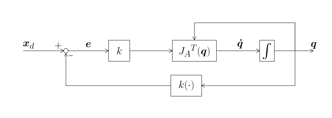
The algorithm only requires the computation of \(J_A^T(\boldsymbol{q})\) and \(k(\cdot)\).
These two algorithms operate on error variables (that contain position and orientation). The error in orientation has to be handled with care; it depends on the representation used.
Euler angles
\(\boldsymbol{\phi}_e\): This is not directly known. We know \(R_e(\boldsymbol{q})\) and from this matrix we can extract \(\boldsymbol{\phi}_e\). In this process there are sign choices to be made.