Differential Kinematics¶

Based on chapter 8 of Robotics, Vision and Control by Peter Corke, and on chapter 3 of Robotics: Modelling, Planning and Control by Siciliano, Sciavicco, Villani and Oriolo.

It uses the The robotics toolbox for MATLAB.

It also uses the MATLAB Symbolic Math Toolbox (functions syms, assume, simplify, diff, subs).

Link to the theoretical session on Kinematics

Geometric Jacobian¶

The anthropomorphic arm¶

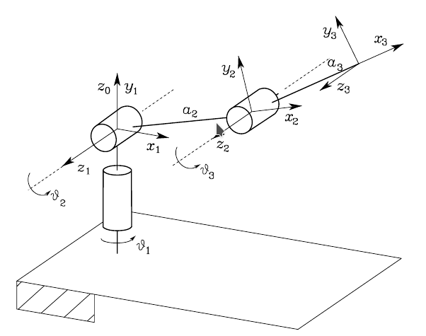
The Jacobian for three revolute joints is:

$J(\mathbf{q}) = \left[ {\begin{array}{c} J_p(\mathbf{q}) \\ J_{\Theta}(\mathbf{q}) \\ \end{array} } \right] = \left[ {\begin{array}{ccc} \mathbf{z}_0 \times (\mathbf{p}_e - \mathbf{p}_0) & \mathbf{z}_1 \times (\mathbf{p}_e - \mathbf{p}_1) & \mathbf{z}_2 \times (\mathbf{p}_e - \mathbf{p}_2) \\ \mathbf{z}_0 & \mathbf{z}_1 & \mathbf{z}_2 \\ \end{array} } \right]$

The homogeneous transformations between links are:

$A_1^{0}(q_1) = \left[ {\begin{array}{cccc} c_1 & 0 & s_1 & 0 \\ s_1 & 0 & -c_1 & 0 \\ 0 & 1 & 0 & 0 \\ 0 & 0 & 0 & 1 \\ \end{array} } \right],\;\;\;\;\; A_i^{i-1}(q_i) = \left[ {\begin{array}{cccc} c_i & -s_i & 0 & a_i c_i \\ s_i & c_i & 0 & a_i s_i \\ 0 & 0 & 1 & 0 \\ 0 & 0 & 0 & 1 \\ \end{array} } \right] \;\;\; i=2,3.$

The origin $\mathbf{\tilde{p}}^i_i=[0\; 0\; 0\; 1]^T$ of the reference frame of link $i\in \{0..3\}$ is represented in the base frame as:

$\mathbf{\tilde{p}}_0 = \left[ {\begin{array}{c} 0 \\ 0 \\ 0 \\ 1 \\ \end{array} } \right],\;\;\; \mathbf{\tilde{p}}_1 = A_1^{0}(q_1)\mathbf{\tilde{p}}^1_1 = \left[ {\begin{array}{c} 0 \\ 0 \\ 0 \\ 1 \\ \end{array} } \right],\;\;\; \mathbf{\tilde{p}}_2 = A_1^{0}(q_1)A_2^{1}(q_2)\mathbf{\tilde{p}}^2_2 = \left[ {\begin{array}{c} a_2 c_1 c_2 \\ a_2 s_1 c_2 \\ a_2 s_2 \\ 1 \\ \end{array} } \right],\;\;\; \mathbf{\tilde{p}}_e =\mathbf{\tilde{p}}_3 = A_1^{0}(q_1)A_2^{1}(q_2)A_3^{2}(q_3)\mathbf{\tilde{p}}^3_3 = \left[ {\begin{array}{c} c_1 (a_2 c_2 + a_3 c_{23}) \\ s_1 (a_2 c_2 + a_3 c_{23}) \\ a_2 s_2 + a_3 s_{23} \\ 1 \\ \end{array} } \right].$

The z-axes of the link reference frames are:

$\mathbf{z}_0 = \left[ {\begin{array}{c} 0 \\ 0 \\ 1 \\ \end{array} } \right],\;\;\; \mathbf{z}_1 = R_1^{0}(q_1)\mathbf{z}_0 = \left[ {\begin{array}{c} s_1 \\ -c_1 \\ 0 \\ \end{array} } \right],\;\;\; \mathbf{z}_2 = R_1^{0}(q_1)R_2^{1}(q_2)\mathbf{z}_0 = \left[ {\begin{array}{c} s_1 \\ -c_1 \\ 0 \\ \end{array} } \right].$

Then, the Jacobian results:

$J(\mathbf{q}) = \left[ {\begin{array}{ccc} -s_1 (a_2 c_2 + a_3 c_{23}) & -c_1 (a_2 s_2 + a_3 s_{23}) & -a_3 c_1 s_{23}\\ c_1 (a_2 c_2 + a_3 c_{23}) & -s_1 (a_2 s_2 + a_3 s_{23}) & -a_3 s_1 s_{23} \\ 0 & a_2 c_2 + a_3 c_{23} & a_3 c_{23}\\ 0 & s_1 & s_1 \\ 0 & -c_1 & -c_1 \\ 1 & 0 & 0 \\ \end{array} } \right]$

Coding with the Matlab symbolic toolbox¶

The previous developments can be coded efficiently using the Matlab Symbolic Toolbox as follows:

clear
%
%joint variables
syms q1
syms q2
syms q3
assume(q1,'real')
assume(q2,'real')
assume(q3,'real')
%link lengths
syms a2
syms a3
assume(a2,'real')
assume(a3,'real')
%A matrices
A01 = [cos(q1) 0  sin(q1) 0;...
       sin(q1) 0 -cos(q1) 0;...
          0    1     0    0;...
          0    0     0    1]
A12 = [cos(q2) -sin(q2) 0  a2*cos(q2);...
       sin(q2)  cos(q2) 0  a2*sin(q2);...
          0       0     1    0;...
          0       0     0    1]
A23 = [cos(q3) -sin(q3) 0  a3*cos(q3);...
       sin(q3)  cos(q3) 0  a3*sin(q3);...
          0       0     1    0;...
          0       0     0    1]
p0 = [0 0 0 1]'
p1 = A01*p0
p2 = A01*A12*p0
p3= A01*A12*A23*p0
z0 = [0 0 1]';
z1 = A01(1:3,1:3)*z0
z2 = A01(1:3,1:3)*A12(1:3,1:3)*z0

J = [ cross(z0,p3(1:3)-p0(1:3)),  cross(z1,p3(1:3)-p1(1:3)),  cross(z2,p3(1:3)-p2(1:3));...
            z0                  z1                z2]
        
J = simplify(J)

Using the robotics toolbox¶

The Robotics Toolbox provides a method in the SerialLink class that allows to compute the Geometric Jacobian at a given configuration:

>> mdl_puma560
>> J = p560.jacob0(qn)

The Geometric Jacobian $J(\mathbf{q})$ relates the joint velocities $\dot{\mathbf{q}}$ with the end-effector linear and angular velocities $\mathbf{v}=(\dot{x},\dot{y},\dot{z},\omega_x,\omega_y,\omega_z)^T$ . The function jacbo0 gives the Cartesian velocities of the end-effector measured from the base frame (hence the 0 in the name of the function)

The rows of J are the Cartesian degrees of freedom and the columns the joints, therefore for the 6 degree of freedom Puma 560 manipulator the Jacobian is a (6x6) square matrix.

The (3x3) zero block indicates that the joint velocities of the wrist joints do not have any effect on the linear motion of the end-effector.

The joint velocities required to move along a small velocity in the z-direction are:

>> qd = inv(J)*[0 0 0.1 0 0 0]'

>>> EXERCISE
  Write a Matlab function called qdot that has as input a serial link, a configuration and a desired operational space velocity and returns the joint velocities.

Analytic Jacobian¶

The anthropomorphic arm¶

The Analytical Jacobian is:

$J_A(\mathbf{q}) = \left[ {\begin{array}{c} J_p(\mathbf{q}) \\ J_{\Phi}(\mathbf{q}) \\ \end{array} } \right] = \left[ {\begin{array}{c} \frac{\partial \mathbf{p}_e}{\partial \mathbf{q}} \\ \frac{\partial \mathbf{\Phi}_e}{\partial \mathbf{q}} \\ \end{array} } \right]$

The position of the end effector is:

$\mathbf{p}_e = \left[ {\begin{array}{c} c_1 (a_2 c_2 + a_3 c_{23}) \\ s_1 (a_2 c_2 + a_3 c_{23}) \\ a_2 s_2 + a_3 s_{23} \end{array} } \right]$

Then, the linear part of the analytical Jacobian becomes:

$J_p(\mathbf{q}) = \left[ {\begin{array}{ccc} \frac{\partial x}{\partial q_1} & \frac{\partial x}{\partial q_2} & \frac{\partial x}{\partial q_3} \\ \frac{\partial y}{\partial q_1} & \frac{\partial y}{\partial q_2} & \frac{\partial y}{\partial q_3} \\ \frac{\partial z}{\partial q_1} & \frac{\partial z}{\partial q_2} & \frac{\partial z}{\partial q_3} \\ \end{array} } \right] = \left[ {\begin{array}{ccc} -s_1 (a_2 c_2 + a_3 c_{23}) & -c_1 (a_2 s_2 + a_3 s_{23}) & -c_1 a_3 s_{23}\\ c_1 (a_2 c_2 + a_3 c_{23}) & -s_1 (a_2 s_2 + a_3 s_{23}) & -s_1 a_3 s_{23}\\ 0 & a_2 c_2 + a_3 c_{23} & a_3 c_{23} \end{array} } \right]$

The orientation of the end effector is:

$\mathbf{\Phi}_e = \left[ \begin{array}{ccc} c_1 c_{23} & -c_1 s_{23} & s_1 \\ s_1 c_{23} & -s_1 s_{23} & -c_1 \\ s_{23} & c_{23} & 0 \end{array} \right] = \left[ \begin{array}{ccc} r_{11} & r_{12} & r_{13} \\ r_{21} & r_{22} & r_{23} \\ r_{31} & r_{32} & r_{33} \\ \end{array} \right]$

The corresponding ZYZ Euler angles are:

$\begin{array}{rcl} \phi & = & \textrm{atan2}(r_{23},r_{13}) = \textrm{atan2}(-c_1,s_1) = q_1 - \frac{\pi}{2}\\ \theta & = & \textrm{atan2}(\sqrt{r_{13}^2 + r_{23}^2}, r_{33}) = \textrm{atan2}(1,0) = \frac{\pi}{2}\\ \psi & = & \textrm{atan2}(r_{32},-r_{31}) = \textrm{atan2}(c_{23},-s_{23}) = q_2+q_3+\frac{\pi}{2}\\ \end{array}$

Then, the angular part of the analytical Jacobian becomes:

$J_\Phi(\mathbf{q}) = \left[ {\begin{array}{ccc} \frac{\partial \phi}{\partial q_1} & \frac{\partial \phi}{\partial q_2} & \frac{\partial \phi}{\partial q_3} \\ \frac{\partial \theta}{\partial q_1} & \frac{\partial \theta}{\partial q_2} & \frac{\partial \theta}{\partial q_3} \\ \frac{\partial \psi}{\partial q_1} & \frac{\partial \psi}{\partial q_2} & \frac{\partial \psi}{\partial q_3} \\ \end{array} } \right] = \left[ {\begin{array}{ccc} 1 & 0 & 0\\ 0 & 0 & 0\\ 0 & 1 & 1\\ \end{array} } \right]$

It can be verified that it corresponds to the angular part of the Geometric Jacobian computed above, which are related through matrix $T_A(\Phi)$ .

$J_\Theta(\mathbf{q}) = T(\Phi) J_\Phi(\mathbf{q}) = \left[ {\begin{array}{ccc} 0 & -s_\phi & c_\phi s_\theta \\ 0 & c_\phi & s_\phi s_\theta \\ 1 & 0 & c_\theta \\ \end{array} } \right] \left[ {\begin{array}{ccc} 1 & 0 & 0\\ 0 & 0 & 0\\ 0 & 1 & 1\\ \end{array} } \right] = \left[ {\begin{array}{ccc} 0 & c_\phi s_\theta & c_\phi s_\theta \\ 0 & -s_\phi s_\theta & -s_\phi s_\theta \\ 1 & c_\theta & c_\theta \\ \end{array} } \right]$

Since $\phi=q_1-\frac{\pi}{2}$ and $\theta=\frac{\pi}{2}$ , then $c_\phi=s_1$ , $s_\phi=-c_1$ , $c_\theta=0$ , and $s_\theta=1$ . Therefore, as expected:

$J_\Theta(\mathbf{q}) = \left[ {\begin{array}{ccc} 0 & s_1 & s_1 \\ 0 & -c_1 & -c_1 \\ 1 & 0 & 0 \\ \end{array} } \right]$

Coding with the Matlab symbolic toolbox¶

The previous developments can be coded efficiently using the Matlab Symbolic Toolbox as follows:

clear
%
%joint variables
syms q1
syms q2
syms q3
assume(q1,'real')
assume(q2,'real')
assume(q3,'real')
%link lengths
syms a2
syms a3
assume(a2,'real')
assume(a3,'real')
%A matrices
A01 = [cos(q1) 0  sin(q1) 0;...
       sin(q1) 0 -cos(q1) 0;...
          0    1     0    0;...
          0    0     0    1]
A12 = [cos(q2) -sin(q2) 0  a2*cos(q2);...
       sin(q2)  cos(q2) 0  a2*sin(q2);...
          0       0     1    0;...
          0       0     0    1]
A23 = [cos(q3) -sin(q3) 0  a3*cos(q3);...
       sin(q3)  cos(q3) 0  a3*sin(q3);...
          0       0     1    0;...
          0       0     0    1]
A03 = A01*A12*A23;

Pe = A03(:,4)
Phie = A03(1:3,1:3)
phi = atan2(Phie(2,3),Phie(1,3))
theta = atan2(sqrt(Phie(1,3)^2+Phie(2,3)^2),Phie(3,3)) 
psi = atan2(Phie(3,2),-Phie(3,1))

dPexdq1 = diff(Pe(1),q1);
dPexdq2 = diff(Pe(1),q2);
dPexdq3 = diff(Pe(1),q3);
dPeydq1 = diff(Pe(2),q1);
dPeydq2 = diff(Pe(2),q2);
dPeydq3 = diff(Pe(2),q3);
dPezdq1 = diff(Pe(3),q1);
dPezdq2 = diff(Pe(3),q2);
dPezdq3 = diff(Pe(3),q3);
Jp = [dPexdq1 dPexdq2 dPexdq3;...
      dPeydq1 dPeydq2 dPeydq3;...
      dPezdq1 dPezdq2 dPezdq3]
Jp = simplify(Jp)


dphidq1 = diff(phi,q1);
dphidq2 = diff(phi,q2);
dphidq3 = diff(phi,q3);
dthetadq1 = diff(theta,q1);
dthetadq2 = diff(theta,q2);
dthetadq3 = diff(theta,q3);
dpsidq1 = diff(psi,q1);
dpsidq2 = diff(psi,q2);
dpsidq3 = diff(psi,q3);
JPhi = [dphidq1 dphidq2 dphidq3;...
      dthetadq1 dthetadq2 dthetadq3;...
      dpsidq1 dpsidq2 dpsidq3]
JPhi = simplify(JPhi)
  
JA = [Jp;JPhi]

Using the robotics toolbox¶

The jacob0 method introduced before, gives us the Analytical Jacobian if the parameter `eul` is added:

>> JA = p560.jacob0(qn,'eul')

The relation between the Geometric Jacobian and the Analytic Jacobian is:

$J = T_A(\Phi_e) J_A = \left[ {\begin{array}{cc} \mathbf{I}_3 & \mathbf{0}_3 \\ \mathbf{0}_3 & T(\Phi_e) \\ \end{array} } \right] J_A$

The Toolbox provides the function eul2jac(phi,theta,psi) that implements the matrix $T(\Phi_e)$ , with $\Phi_e$ being the ZYZ Euler angles $\Phi_e = [\phi,\theta,\psi]^T$ .

>> Tn = p560.fkine(qn)
>> Phi_e = Tn.toeul
>> TA = J*inv(JA)
>> T = TA(4:6,4:6)
>> T = eul2jac(Phi_e)

Alternatively to the use of ZYZ Euler angles, RPY angles can be used, and then the expression of the analytical Jacobian and that of matrix $T(\Phi_e)$ vary. Matrix $T(\Phi_e)$ is implemented in the robotics toolbox by the function rpy2jac.

Singularities / Manipulability¶

If we compute the Jacobian at configuration qr we see that the columns 4 and 6 are identical, meaning that motions of these joints will produce the same Cartesian motion:

>> J = p560.jacob0(qr)
>> rank(J)
>> det(J)

The singularity check can be done by the following function:

>> jsingu(J)

Let’s analyze what happens near the singularities, by slightly changing to a configuration near qn:

>> q = qn
>> q(5) = 5*pi/180
>> J = p560.jacob0(q)
>> rank(J)
>> det(J)
>> jsingu(J)

In this configuration the velocities required to move along a small velocity in the z-direction are very large (compare them with qd, the joint velocities obtained in configuration qn computed in the first section):

>> qd2 = inv(J)*[0 0 0.1 0 0 0]'

Near singularities the manipulability is small. This can be visualized using the translational and angular velocity ellipsoids:

>> Jt = J(1:3,:)
>> plot_ellipse(Jt*Jt')
>> Ja = J(4:6,:)
>> figure
>> plot_ellipse(Ja*Ja')

The manipulability index $\sqrt{det(J,J')}$ is computed as follows:

>> mt_q = p560.maniplty(q,'yoshikawa','trans')
>> mr_q = p560.maniplty(q,'yoshikawa','rot')

The following source code illustrates how the manipulability changes for different configurations of a two-link planar arm performing a two-degrees of freedom planar task. Note that only the degrees of freedom of the task (r=2) are taken into account, i.e. the Jacobian used to compute the manipulability is of dimension $r\times n = 2\times 2$ .

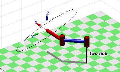
>>> EXERCISE
  Change the configuration in the script to visualize the manipulability ellipsoid in different regions of the workspace.

Redundancy¶

Consider the redundant mobile manipulator p8 consituted by a xy platform and the Puma 560 robot.

>> qn8 = [0, 0, qn]
>> platform = SerialLink( [0 0 0 -pi/2 1; -pi/2 0 0 pi/2 1], 'base', troty(pi/2), 'name', 'platform' )
>> p8 = SerialLink([platform, p560])
>> J = p8.jacob0(qn8)
>> about(J)

We have to use the pseudoinverse to compute the required $\dot{q}$ for a given desired end-effector velocity $\omega_e$ . The pseudoinvese $J ^\dagger = J^T(J^T J)^{-1}$ is computed by function pinv:

>> xd = [0.2 0.2 0.2 0 0 0]'
>> qd = pinv(J)*xd

Redundancy can be used to achieve motions that satisfy a secondary objective like maximizing manipulability.

$\dot{\mathbf{q}} = J^\dagger \mathbf{v}_e + (I_n - J^\dagger J) \dot{\mathbf{q}}_0 \dot{\mathbf{q}}_0 = k_0\left (\frac{\partial \omega(\mathbf{q})}{\partial \mathbf{q}} \right )^T \omega(\mathbf{q}) = \sqrt{det(J(\mathbf{q})J^T(\mathbf{q}))}$

Consider now a planar manipulator with three joints performing a two-degrees-of-freedom planar task (only the position of the end effector is relevant, not its orientation). The following source code illustrates the use of redundancy to move the tree-link planar arm along an operational space velocity while maximizing manipulability:

The file threeLink.m executes and plots a motion.

The file threeLinkJacobianTest.m computes symbolically the Jacobian and tests it.

The file threeLinkJacobian.m stores the final expression of the Jacobian, which is used by the script threeLink.m.

EXERCISE (Deliverable)¶

>>> Exercise A
  Compute the Geometric Jacobian of the spherical wrist

>>> Exercise B
  Compute the Analytical Jacobian of the spherical wrist. Verify that it is related with the Geometric Jacobian by matrix T_A.

>>> Exercise C
  Modify the file *threeLink.m* to compute the manipulability all along the motion, and compare it for a trajectory generated when no maximization of the manipulability is considered.

>>> Exercise D (optional)
  Compute the Jacobian of the UR3 robot using the DH parameters provided by Universal Robots.

Differential Kinematics¶

Geometric Jacobian¶

The anthropomorphic arm¶

Coding with the Matlab symbolic toolbox¶

Using the robotics toolbox¶

Analytic Jacobian¶

The anthropomorphic arm¶

Coding with the Matlab symbolic toolbox¶

Using the robotics toolbox¶

Singularities / Manipulability¶

Redundancy¶

EXERCISE (Deliverable)¶

Table of Contents

Previous topic

Next topic