Kinematics¶

Based on chapter 7 of Robotics, Vision and Control by Peter Corke, and on chapter 2 of Robotics: Modelling, Planning and Control by Siciliano, Sciavicco, Villani and Oriolo.

It uses the The robotics toolbox for MATLAB.

It also uses the MATLAB Symbolic Math Toolbox (functions syms, assume, simplify, subs).

Link to the theoretical session on Kinematics

Forward kinematics¶

The two link planar robot¶

Use the script provided by the toolbox to load the two-link planar robot, and change the base so as to move on the XY plane:

>> mdl_twolink
>> twolink
>> twolink.base = transl(0,0,0)

Compute the forward kinematics and plot:

>> twolink.fkine([0,0])
>> twolink.plot([0,0])
>> twolink.fkine([pi/4,pi/4])
>> twolink.plot([pi/4,pi/4])

The PUMA 560 robot¶

Use the script provided by the toolbox to load the PUMA 560 robot and the frequently used configurations qz, qr, qs and qn:

>> mdl_puma560
>> p560
>> p560.plot(qz)
>> p560.plot(qr)
>> p560.plot(qs)
>> p560.plot(qn)

Compute the forward kinematics at qz using the fkine method that returns an SE3 element. Clone the robot and repeat after defining a Tool and a Base for the new robot. Verify the differences in the homogeneous transforms.

>> T1 = p560.fkine(qz)
>> p560b = SerialLink(p560, 'name', 'Puma 560b');
>> p560b.tool = transl(0,0,0.2)
>> T2 = p560b.fkine(qz)
>> p560b.base = transl(0,0,1)
>> T3 = p560b.fkine(qz)
>> p560.plot(qz)
>> figure
>> p560b.plot(qz, 'workspace', [-1,1,-1,1,-1,2])

Coding with the Matlab symbolic toolbox¶

The forward kinematics can be coded efficiently using the Matlab Symbolic Toolbox as follows.

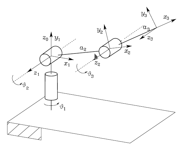
As an example, the forward kinematics of the anthropomorphic arm is:

clear
%joint variables
syms qi q1 q2 q3
assume(qi,'real')
assume(q1,'real')
assume(q2,'real')
assume(q3,'real')
%link lengths
syms ai a2 a3
assume(ai,'real')
assume(a2,'real')
assume(a3,'real')
%link offsets
syms di
assume(di,'real')
%link twists
syms alphai
assume(alphai,'real')

%%%%%%%%%%%%%%%%%%%%%%%%%%%%%%%%%%%%%%%%%%%%%%%%%%%%%%%%%%%%%%%%
%% MODELLING
%A matrices
A01i = [cos(qi) -sin(qi)*cos(alphai)  sin(qi)*sin(alphai) ai*cos(qi);...
       sin(qi)  cos(qi)*cos(alphai) -cos(qi)*sin(alphai) ai*sin(qi);...
          0     sin(alphai)          cos(alphai)         di;...
          0    0     0    1]
    
A01 = subs(A01i,{ai,di,alphai,qi},{  0,    0,  pi/2, q1})
A12 = subs(A01i,{ai,di,alphai,qi},{ a2,    0,     0, q2})
A23 = subs(A01i,{ai,di,alphai,qi},{ a3,    0,     0, q3})

%%%%%%%%%%%%%%%%%%%%%%%%%%%%%%%%%%%%%%%%%%%%%%%%%%%%%%%%%
%% DIRECT KINEMATICS
A03 = A01*A12*A23
simplify(A03)

>>> EXERCISE
    Particularize for an arm with link lengths equal to 1, compute the forward kinematics for [pi/4, pi/3, pi/2] and check the result using the robotics toolbox.

The solution can downloaded from here.

>>> EXERCISE
    - Repeat for the spherical wrist.
    - Particularize for a wrist with d6=1.0, compute the forward kinematics for [pi/4, pi/3, pi/2] and check the result using the robotics toolbox.

The solution can downloaded from here.

>>> EXERCISE
    - Repeat for the spherical arm.
    - Particularize for an arm with link lengths equal to 1, compute the forward kinematics for [pi/4, pi/3, pi/2] and check the result using the robotics toolbox.

>>> EXERCISE
    - Repeat for the two-link planar arm.
    - Particularize for the arm geometry of the twolink robot, compute the forward kinematics for [pi/4,pi/4] and check the result using the robotics toolbox.

>>> EXERCISE
    - Repeat for the UR5 robot.
    - Particularize for the arm geometry, compute the forward kinematics for [0 0 0 0 0 0] and check the result using the robotics toolbox.

Inverse kinematics¶

Anthropomorphic arm¶

Closed form solution¶

We will follow an algebraic solution to obtain the IK of this manipulator.

Theta_3

Consider the position of point W located at the origin of frame 3:

Squaring and summing:

Then:

The solution is admissible if $-1\leq c_3\leq 1$ , i.e. if W lies within the reachable workspace $|a_2-a_3|\leq \sqrt{P^2_{w_x}+P^2_{w_y}+P^2_{w_z}}\leq |a_2+a_3|$ .

Then:

Theta_2

From the expression of $P_{w_x}$ and $P_{w_y}$ :

Together with $P_{w_z}$ the following system of equation will allow us to compute $\theta_2$ :

The sine and cosine of $\theta_2$ are:

Finally:

Theta_1

The expression of $P_{w_x}$ and $P_{w_y}$ can be rewritten as:

Then:

Solutions

The IK of the arm has four solutions:

../_images/IK_solution_anthropomorphic_arm.png

Code¶

>>> EXERCISE
    - Code the IK of the anthropomorphic arm using the Symbolic Toolbox
    - Particularize for an arm with link lengths equal to 1, compute the inverse kinematics for the position of the EE corresponding to the joint values [pi/4, pi/3, pi/2].
    - Check the result using the robotics toolbox.

The solution can downloaded from here.

Spherical wrist¶

Closed form solution¶

From the forward kinematics:

and considering the rotation matrix of the spherical wrist homogeneous transform as:

the expressions of $\theta_5$ , $\theta_4$ and $\theta_6$ can be derived:

Code¶

>>> EXERCISE
    - Code the IK of the spherical wrist using the Symbolic Toolbox
    - Particularize for a wrist  with d6=0, compute the inverse kinematics for the orientation of the EE corresponding to the joint values [pi/4, pi/3, pi/2].
    - Check the result using the robotics toolbox.

The solution can downloaded from here.

Anthropomorphic arm with a spherical wrist¶

Closed form solution procedure¶

A six-DOF manipulator has a closed-form solution if:

Three consecutive joints intersect at a common point (like in the case of the spherical wrist),
Three consecutive revolute joint axes are parallel.

In the case of a manipulator with a spherical wrist, the solution is decoupled between position and orientation, i.e. the three joints of the arm are used to position the end-effector, and the three joints are used to fix its orientation.

../_images/manip_with_spherical_wrist.png

Given the end-effector position $\mathbf{p}_e$ and orientation $R_e$ , the following steps should be followed:

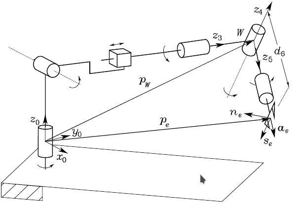
Compute the wrist position $\mathbf{p}_W = \mathbf{p}_e - d_6\mathbf{a}_e$ (see figure).
Solve inverse kinematics for Anthropomorphic arm: $\theta_3,\theta_2,\theta_1$ .
Compute $R_3^0(\theta_1,\theta_2,\theta_3)$
Compute $R_6^3(\theta_4,\theta_5,\theta_6) = {R_3^0}^T R_e$
Solve inverse kinematics for Spherical wrist: $\theta_4,\theta_5,\theta_6$ .

The four solutions of the IK of the arm combined with the two solution of the wrist give a total of eight solutions.

Code¶

>>> EXERCISE
    - Code the IK of the anthropomorphic arm using the Symbolic Toolbox.
    - Particularize for an arm with link lengths (a2 and d4 in the figure below) equal to 1 and d6=0.1, compute the inverse kinematics for the position of the EE corresponding to the joint values [pi/4, pi/3, pi, pi/4, pi/3, pi/2].
    - Check the result using the robotics toolbox.

To solve the exercise note that frame 3 has to be located in a different place in comparison to when the arm was considered alone. Before it was located at the end effector with $z_3$ axis arbitarily set parallel to $z_2$ . Now, when considereing also the wrist, $z_3$ must be along the $\theta_4$ joint axis and the origin of the frame at the intersection of $z_2$ and $z_3$ , as shown in the figure below. The link lenght previously defined by $a_3$ is now defined by $d_4$ , and $\alpha_3$ is now $\frac{\pi}{2}$ , as shown in the table of DH parameters shown below.

As a consequence, the expressions of the inverse kinematics for the arm presented above should be modified for joint $\theta_3$ by a $\pi/2$ offset.

Using the robotics toolbox¶

Closed form solutions¶

The ikine6s function of the SerialLink class gives a closed form solution of the inverse kinematics for six DOF manipulators with spherical wrist like the Puma 560:

>> qn
>> T = p560.fkine(qn)
>> q1 = p560.ikine6s(T)

Note that q1 is different from qn.

The eight different inverse kinematic solutions can be obtained by specifying:

r/l: right arm / left arm.
u/d: elbow up / elbow down.
f/n: flipped wrist / not flipped wrist.

The default values are: l, u and n.

>> q2 = p560.ikine6s(T, 'ru')

>>> EXERCISE
    Check the other solutions solutions and plot them.

Numerical solutions¶

The ikine function of the SerialLink class gives a numerical solution using differential kinematics, and therefore is useful for any kind of manipulators.

>> qn
>> T = p560.fkine(qn)
>> q1 = p560.ikine(T)

Note that the solution q1 is different from qn. In this case the solution found has the elbow down. With this numerical solution, the solution found depends on the initial configuration (which is defaulted to zero), and can not be explicitly controlled although different solutions can be found by changing the initial configuration:

>> q2 = p560.ikine(T, 'q0', [0 0 3 0 0 0])

Under-actuated manipulators¶

Under-actuated manipulator have fewer than six joints, and is therefore limited in the end-effector poses that it can attain.

The ikine method allows us to consider only error in some of the coordinates and ignore all other degrees of freedom, e.g. for the two-link planar manipulator only error in the x- and y-axis translational directions will be considered. This is done by a mask parameter is used to specify the Cartesian DOF (in the wrist coordinate frame) that will be ignored in reaching a solution. The mask vector has six elements that correspond to translation in X, Y and Z, and rotation about X, Y and Z respectively (the value should be 0 for ignore or 1 otherwise).

>> mdl_twolink
>> T = transl(0.4, 0.5, 0.6);
>> q = twolink.ikine(T, 'q0', [0 0], 'mask', [1 1 0 0 0 0])

Redundant manipulators¶

The ikine function can also be used for redundant manipulators.

To illustrate this, consider the Puma 560 robot with a mobile xy base. The translational degrees of freedom of the base can be defined as two prismatic joints:

First define the platform:

>> platform = SerialLink( [0 0 0 -pi/2 1; -pi/2 0 0 pi/2 1], 'base', troty(pi/2), 'name', 'platform' )
>> platform.fkine([1,2])

Then put the Puma 560 on the platform using a 1 m pedestal. To do this, the $d$ parameter of link 1 has to be modified (here we cannot add a base to the Puma 560 because this can only be done at the start of the kinematic chain and now the chain will start with the two prismatic links).

>> p560.links(1).d = 1
>> p8 = SerialLink([platform, p560])

Now, define a given pose and move the mobile manipulator to place its tool there:

>> T = transl(1.0, 1.0, 1.7)*rpy2tr(0,3*pi/4,0)
>> q1 = p8.ikine(T)
>> p8.plot(q1,'workspace',[0,3,0,3,-1,2],'tilesize',1.0,'scale',0.3)

>>> EXERCISE
      Change the initial configuration and verify that different solutions are obtained.

Kinematics¶

Forward kinematics¶

The two link planar robot¶

The PUMA 560 robot¶

Coding with the Matlab symbolic toolbox¶

Inverse kinematics¶

Anthropomorphic arm¶

Closed form solution¶

Code¶

Spherical wrist¶

Closed form solution¶

Code¶

Anthropomorphic arm with a spherical wrist¶

Closed form solution procedure¶

Code¶

Using the robotics toolbox¶

Closed form solutions¶

Numerical solutions¶

Under-actuated manipulators¶

Redundant manipulators¶

Table of Contents

Previous topic

Next topic