Modelling

Based on chapter 2 and chapter 7 of Robotics, Vision and Control by Peter Corke, and on chapter 2 of Robotics: Modelling, Planning and Control by Siciliano, Sciavicco, Villani and Oriolo.

It uses the The robotics toolbox for MATLAB.

Link to the theoretical session on Robot Modelling

Preliminaries

Attention

The robotics toolbox uses radians for the angles but, depending on which toolboxes are installed and in which order, it may interpret angles in degrees, which will produce erroneous results.

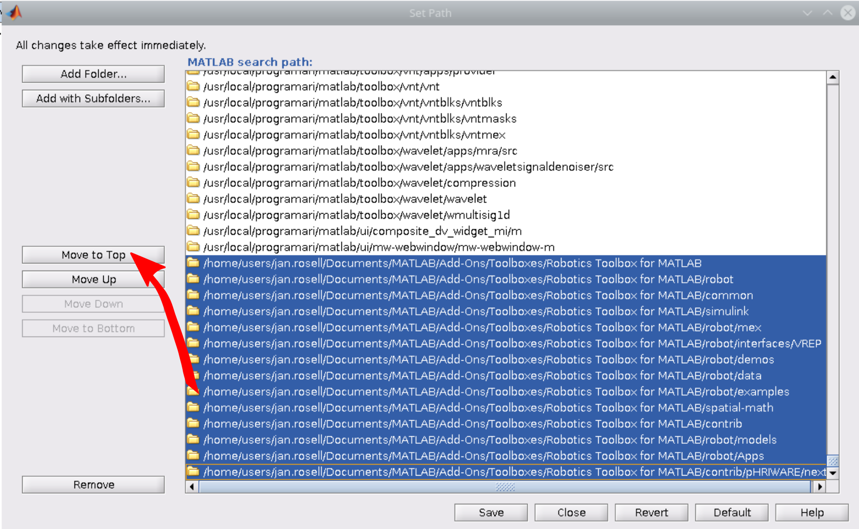
To avoid this, from the menu Environment->SetPath, move the robotics Toolbox to the top of the Path list as shown in the figure:

Basic commands for representing position and orientation

Rotation matrices

R = rotx(pi/2)
trplot(R)
tranimate(R)
R = rotx(pi/2) * roty(pi/2)
trplot(R)

Euler angles ZYZ

Euler angles ZYZ (\([\phi,\theta,\psi]\)) correspond to rotations about moved axes. The equivalent rotation matrix is \(R = R_z(\phi)R_{y'}(\theta)R_{z''}(\psi)\):

R = rotz(0.1)*roty(0.2)*rotz(0.3)
R = eul2r(0.1,0.2,0.3)
gamma = tr2eul(R)

Exercise

Repeat with theta=-0.2. Note that a different set of Euler angles is returned, i.e. different sets of Euler angles give the same rotation matrix.

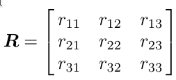
The expression of the rotation matrix as a function of the ZYZ-Euler angles is:

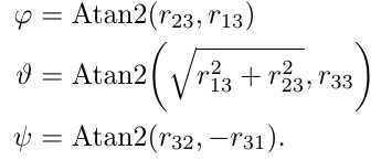
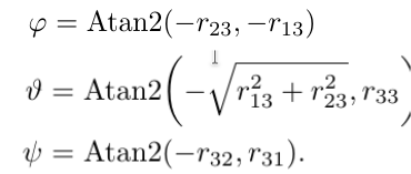
And the inverse problem is:

Euler angles RPY

Euler angles RPY (\([\theta_{roll},\theta_{pitch},\theta_{yaw}]\)) correspond to rotations about fixed axes: first \(\theta_{yaw}\) about \(x^W\), then \(\theta_{pitch}\) about \(y^W\), finally \(\theta_{roll}\) about \(z^W\),. The equivalent rotation matrix is \(R = R_z(\theta_{roll})R_y(\theta_{pitch})R_x(\theta_{yaw})\)

R = rotz(0.3)*roty(0.2)*rotx(0.1)
R = rpy2r(0.1,0.2,0.3,'zyx')
gamma = tr2rpy(R, 'zyx')

Since from version 10 of the Toolbox the ‘zyx’ is the default option, it could be omitted. If, instead, the parameter ‘xyz’ is passed to the rpy2r function then it considers a different definition of the RPY angles where the roll is about the x axis and the yaw about the z axis, i.e. \(R = R_x(\theta_{roll})R_y(\theta_{pitch})R_z(\theta_{yaw})\).

The expression of the rotation matrix as a function of the RPY-Euler angles is:

And the inverse problem is:

Axis-angle

R = angvec2r(pi/2,[1 0 0])
[theta,v] = tr2angvec(R)

The expression of the rotation matrix as a function of the angle and axis is:

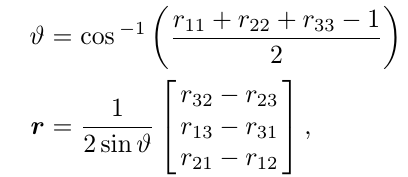
And the inverse problem is:

Quaternion

help UnitQuaternion
q1 = UnitQuaternion(R)
q1.R
q2 = q1.inv
q=q1*q2
q.R

The expression of the rotation matrix as a function of the quaternion is:

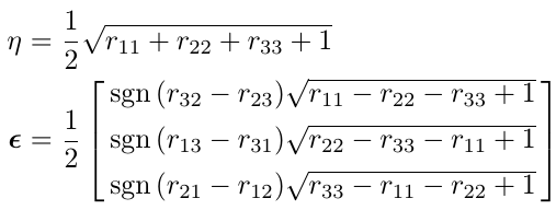
And the inverse problem is:

Conversion functions

The following figure shows the conversion between all rotational representations offered by the Robotics Toolbox.

Homogeneous Transformations

The following functions create (4x4) matrices that represent homogeneous transformations:

T1 = transl(1, 0 ,0)
T2 = trotx(pi/2)
T = T1*T2
trplot(T)
R=t2r(T)
p=transl(T)

SE3

A class named SE3 is also provided to represent homogeneous transformations. It has many constructor methods, operators and also many operation, conversion, information methods:

TT1 = SE3(1,0,0)
TT2 = SE3.Rx(pi/2)
TTa = SE3(T)
about(T)
about(TTa)
TTb = TT1*TT2
res = TTa*TTb.inv
res.isidentity
help SE3

Robot modelling using DH parameters

The modelling of robotic manipulators is done as follows using the Robotics Toolbox:

Link parameters

A link is defined with the function Link:: \(L = Link(\theta,d,a,\alpha)\);

Two additional parameters can be added to specify the type of joint (0/1: revolute/prismatic, with default to 0) and the type of parameters (0/1: standard/modified, with default to 0). Other more explicit constructors are also provided (see the help for details):

help Link
L = Link([0, 0.1, 0.2, pi/2])
L = Link('revolute', 'd', 0.1, 'a', 0.2, 'alpha', pi/2);
L = Revolute('d', 1.2, 'a', 0.3, 'alpha', pi/2);

You can retrieve the link information and also evaluate the link frame for a given joint value (e.g. \(q=0.5\)):

L.type()
L.a
L.A(0.5)

Add an offset to the joint angle and evaluate again:

L.offset = 0.5
L.A(0)

A two-link planar robot

Consider a two-link planar arm with the following DH parameters:

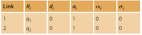
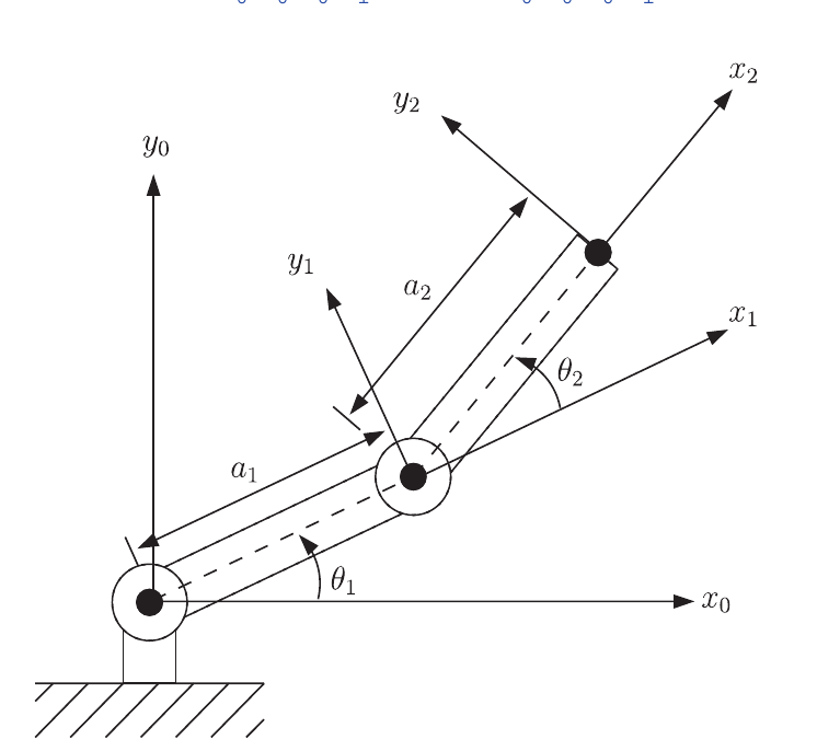
A function called SerialLink allows us to define kinematic structures:

L(1) = Link([0 0 1 0]);
L(2) = Link([0 0 1 0]);
L
twolink = SerialLink(L, 'name', 'two link')

Another manipulator can be create from an existing one:

clone = SerialLink(twolink,'name','twin')

The manipulator can be ploted and interactively moved:

help SerialLink
twolink.plot([0,0])
twolink.teach

Some few robot models are already available in the Toolbox, that can be instantiated just by running a script, thus avoiding the need to create them:

clear
mdl_twolink
twolink.n
L = twolink.links
twolink.display

Procedure to determine the DH parameters

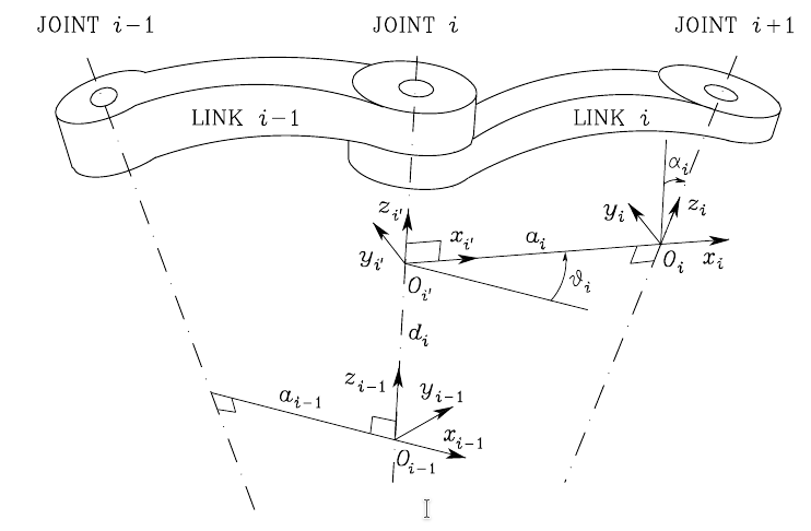
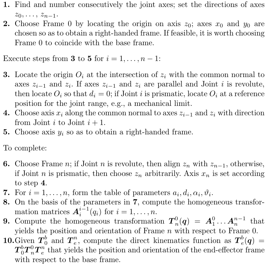
EXERCISE (Deliverable)

Obtain the model the UR5 robot (Universal Robots): Draw the link frames and give the DH table of parameters, including the offsets so as to match the configuration shown in the figure when at configuration [0,0,0,0,0,0] (the home configuration). Create the corresponding SerialLink and plot it at configuration [0,0,0,0,0,0].

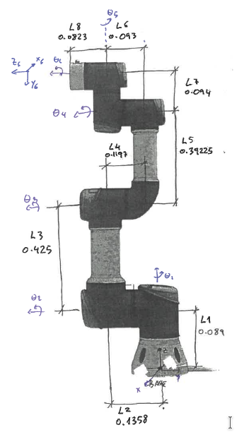
Mandatory: You must do the deliverable with a Live Script using the MATLAB Live Editor. This will allow you to combine text and Matlab code (also, drawings of the frames can be done by hand and inserted in the Live Script as images).