Dynamics

Based on chapter 9 of Robotics, Vision and Control by Peter Corke, and on chapter 7 of Robotics: Modelling, Planning and Control by Siciliano, Sciavicco, Villani and Oriolo.

It uses the The robotics toolbox for MATLAB.

Link to the theoretical session on Dymanics

Equations of motion

The robotics toolbox implements the dynamic equations using the Newton-Euler method, which is computationally efficient. The SerialLink class has several functions to obtain the inverse and the forward dynamics, and the different terms of the equations of motion.

\[B(\mathbf{q})\mathbf{\ddot{q}} + C(\mathbf{q},\mathbf{\dot{q}}) \mathbf{\dot{q}} + F \mathbf{\dot{q}} + g(\mathbf{q}) = \mathbf{\tau}\]

The derivation of these terms will also be done in this tutorial using the symbolic toolbox following the Lagrange method.

The dynamic parameters of the robot are stored in each link. They include the mass, the center of mass, the inertia, the motor inertia, the motor friction and the gear ratio.

mdl_puma560
p560.links(1).dyn
p560.links(6).dyn

Inverse Dynamics

The function rne gives the set of joint torques required to achieve a given configuration, velocity and acceleration. If zero velocity and acceleration are specified, the torques obtained are those required to hold the robot up against gravity.

Qn1 = p560.rne(qn,[0 0 0 0 0 0],[0 0 0 0 0 0])

The required torques to follow a desired trajectory are computed as follows:

q = jtraj(qz, qr,10)
Q = p560.rne(q,0*q,0*q)

Q is a 10x6 matrix containing the torques required at each time step.

The gravity vector being used is:

p560.gravity

The rne function also allows to specify a different gravity vector passing it as a parameter, which is useful if for instance the robot is fixed on the ceiling. We can check that in a zero-gravity environment the resulting required torques are zero:

Qz = p560.rne(qz,[0 0 0 0 0 0],[0 0 0 0 0 0],[0 0 0])

Finally, let’s analyze the torques required at qn when the velocity of the first joint is set to 1 rad/s (with zero acceleration on all joints and without considering gravity):

>>Qn2 = p560.rne(qn,[1 0 0 0 0 0],[0 0 0 0 0 0],[0 0 0])

We can see that, besides torques on joint 1, torques on joints 2, 3 and 4 are also required due to the centripedal and Coriolis forces.

Forward Dynamics

Forward dynamics \(\mathbf{\ddot{q}} = B^{-1}(\mathbf{q}) (\mathbf{\tau} - C(\mathbf{q},\mathbf{\dot{q}}) \mathbf{\dot{q}} - F \mathbf{\dot{q}} - g(\mathbf{q}))\) is implemented with the function accel:

qdd = p560.accel(q, qd, Q)

The function gives the joint accelerations that result from applying the actuator torques Q to the manipulator in the state (q, qd). It has to be used in conjunction with numerical integration in order to simulate the manipulator dynamics.

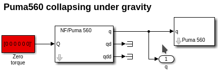
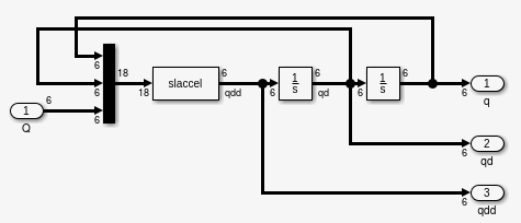
The following Simulink model simulates the collapsing of the puma560 robot under gravity when zero torques are applied. The NF/Puma560 block contains the forward dynamics and the integration:

sl_ztorque

Exercise

Change the input torque to Qn1 (in the Zero torque block) and the initial state to qn (in the NF/Puma560 block) and verify that the computed torque effectively holds the robot at qn against gravity.

Inertia Matrix

The inertia matrix can be obtained by the function inertia:

B = p560.inertia(qn)

Observe that:

B is symmetric,

The diagonal terms describe the inertia seen by the joints, i.e. \(Q_j=B_{jj}\mathbf{\ddot{q}_j}\), and therefore the \(B_{11}\) and \(B_{22}\) terms are greater since they correspond to the heavier links,

The off-diagonal terms represent the couplings.

Effect of payload

If a payload is added at the end-effector (e.g. at distance of 0.1 m in the z-direction), then the inertia matrix varies:

p560.payload(2.5, [0 0 0.1])
Bloaded = p560.inertia(qn)

We can see that the diagonal components have increased significantly, which means that the maximum acceleration allowed will be reduced (and thus it will be more difficult to follow high-speed trajectories). Also, we can see that the inertia of joint 6 is unaffected since the added mass lies in the axis of this joint.

Coding with the Matlab symbolic toolbox

Consider the two-link planar manipulator moving on the xy-plane (with the gravity in the -y direction):

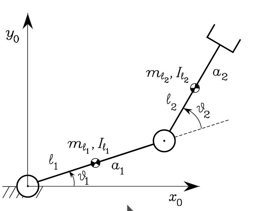
The file two_link_manipulator.m includes the definition of symbolic variables and the modelling of the two-link manipulator using both symbolic expressions and the default twolink model of the Robotics Toolbox that has been modified to include inertia, friction values and gear ratios.
The file two_link_inertia.m includes the computation of the inertia matrix B:

\[\begin{split}B(\mathbf{q}) = \sum_{i=1}^2 [m_{l_i} J_P^{l_i T}(\mathbf{q})J_P^{l_i}(\mathbf{q}) + J_\theta^{l_i T}(\mathbf{q})R_i I_{l_i}^i R_i^T J_\theta^{l_i}(\mathbf{q})]\\ J_P^{l_1}(\mathbf{q}) = \left[ {\begin{array}{cc} -l_1 s_1 & 0 \\ l_1 c_1 & 0 \\ 0 & 0 \end{array} } \right] \;\;\;\; J_P^{l_2}(\mathbf{q}) = \left[ {\begin{array}{cc} -a_1 s_1 - l_2 s_{12} & -l_2 s_{12} \\ a_1 c_1 + l_2 c_{12} & l_2 c_{12} \\ 0 & 0 \end{array} } \right] \;\;\;\; J_\Theta^{l_1}(\mathbf{q}) = \left[ {\begin{array}{cc} 0 & 0 \\ 0 & 0 \\ 1 & 0 \end{array} } \right] \;\;\;\; J_\Theta^{l_2}(\mathbf{q}) = \left[ {\begin{array}{cc} 0 & 0 \\ 0 & 0 \\ 1 & 1 \end{array} } \right]\end{split}\]

%%%%%%%%%%%%%%%%%%%%%%%%%%%%%%%%%%%%%%%%%%%%%%%%%%%%%%%%
%% INERTIA MATRIX
A01_l = subs(A01i,{ai,di,alphai,qi},{ l1, 0, 0, q1})
A12_l = subs(A01i,{ai,di,alphai,qi},{ l2, 0, 0, q2})
pl1 = A01_l*origin
pl2 = A01*A12_l*origin
JP_l1 = [cross(z0,pl1(1:3)-p0(1:3)), [0 0 0]']
JP_l2 = [cross(z0,pl2(1:3)-p0(1:3)), cross(z1,pl2(1:3)-p1(1:3))]
Jtheta_l1 = [z0 [0 0 0]']
Jtheta_l2 = [z0 z1]

B1 = m1*JP_l1'*JP_l1;
B2 = m2*JP_l2'*JP_l2;

R1 = A01(1:3,1:3)
vIl11 = subs(Il11,{Ixx1 Iyy1 Ixy1 Ixz1 Iyz1},{0 0 0 0 0})
Il1 = R1*vIl11*R1'

R2 = A01(1:3,1:3)*A12(1:3,1:3)
vIl22 = subs(Il22,{Ixx2 Iyy2 Ixy2 Ixz2 Iyz2},{0 0 0 0 0})
Il2 = R2*vIl22*R2'

B3 = Jtheta_l1'*Il1*Jtheta_l1
B4 = Jtheta_l2'*Il2*Jtheta_l2

B = simplify(B1+B2+B3+B4)

Execute the scripts:

two_link_manipulator
two_link_inertia

Exercise

Create a script called verification.m. Use function subs to substitute in the expression of B the values of the model and check, for configurations qa=[pi/3 pi/3] and qb=[pi/4 pi/4], that the same is obtained by using the inertia function of the SerialLink class.

Coriolis Matrix

The Coriolis matrix contains the centripetal terms (proportional to \(\mathbf{\dot{q_j}^2}\)) and the Coriolis terms (proportional to \(\mathbf{\dot{q_i}\dot{q_j}}\)), and can be obtained by the function coriolis. Considering the robot at configuration \(q_n\) with velocity \(\dot{q} = 0.5\) for all the joints, then the Coriolis matrix is:

mdl_puma560
qd = 0.5*[1 1 1 1 1 1]
C = p560.coriolis(qn,qd)

Observe that \(C_{1,2}=-0.6453\) is the coupling from joint 2 velocity to torque on joint 1, i.e. rotation of the shoulder exerts a torque on the waist.

The joint torques due to these centripedal and coriolis effects are:

C*qd'

Coding with the Matlab symbolic toolbox

For the two-link planar manipulator moving on the xz-plane:

The file two_link_coriolis.m includes the computation of the Coriolis matrix C:

\[\begin{split}C(\mathbf{q}, \mathbf{\dot{q}}) = \left[ {\begin{array}{cc} c_{11} & c_{12} \\ c_{21} & c_{22} \end{array} } \right] \;\;\;\;\;\;\;\; c_{ij} = \sum_{i=1}^2 c_{ijk} \mathbf{\dot{q}_k}\;\;\;\;\;\;\;\; c_{ijk} = \frac{1}{2}(\frac{\partial b_{ij}}{\partial q_k} + \frac{\partial b_{ik}}{\partial q_j} - \frac{\partial b_{jk}}{\partial q_i})\end{split}\]

%%%%%%%%%%%%%%%%%%%%%%%%%%%%%%%%%%%%%%%%%%%%%%%%%%%%%%%%
%% CORIOLIS MATRIX

%Coriolis and centrifual terms
b11 = B(1,1)
b12 = B(1,2)
b21 = B(2,1)
b22 = B(2,2)
%cijk = simplify(0.5*(diff(bij,qk) + diff(bik,qj)-diff(bjk,qi)))
c111 = simplify(0.5*(diff(b11,q1) + diff(b11,q1)-diff(b11,q1)))
c112 = simplify(0.5*(diff(b11,q2) + diff(b12,q1)-diff(b12,q1)))
c121 = c112
c122 = simplify(0.5*(diff(b12,q2) + diff(b12,q2)-diff(b22,q1)))
c211 = simplify(0.5*(diff(b21,q1) + diff(b21,q1)-diff(b11,q2)))
c212 = simplify(0.5*(diff(b21,q2) + diff(b22,q1)-diff(b12,q2)))
c221 = c212
c222 = simplify(0.5*(diff(b22,q2) + diff(b22,q2)-diff(b22,q2)))

c11 = c111*qdot1+c112*qdot2
c12 = c121*qdot1+c122*qdot2
c21 = c211*qdot1+c212*qdot2
c22 = c221*qdot1+c222*qdot2

C = [c11 c12; c21 c22]

Execute the script:

two_link_coriolis

Exercise

Complete the verification.m script. Substitute in the expression of C the values of the model and check, for configurations qa=[pi/3 pi/3] and qb=[pi/4 pi/4], that the same is obtained by using the coriolis function of the SerialLink class. Use the velocity qd=[0.1 0.1].

Gravity Term

The gravity term gives the required torques to compensate the gravity at a given configuration. It is the dominant term in the dynamic equations (and it is always there!). The function gravload computes this term:

p560.gravload(qn)

We can see that it is the same as the Qn1 torque computed in the Inverse dynamics section. We can check that for the arm at qs (i.e. completely stretched), the required components of the gravity term are higher:

p560.gravload(qs)

Coding with the Matlab symbolic toolbox

For the two-link planar manipulator moving on the xz-plane:

The file two_link_gravity.m includes the computation of the gravity term:

\[\begin{split}\mathbf{g}_0 = [ 0\; -g \; 0]\\ \mathbf{g}(\mathbf{q}) = [g_{1}(\mathbf{q}) \; g_{2}(\mathbf{q})] \\ g_{1}(\mathbf{q}) = -\sum_{j=1}^2 m_{l_j}\mathbf{g}_0^T J_{P_1}^{l_j} \\ g_{2}(\mathbf{q}) = -\sum_{j=1}^2 m_{l_j}\mathbf{g}_0^T J_{P_2}^{l_j}\end{split}\]

%%%%%%%%%%%%%%%%%%%%%%%%%%%%%%%%%%%%%%%%%%%%%%%%%%%%%%%%
%% GRAVITATIONAL TERM

%gravitational term
g0 = [0 -g 0]'
g1 = simplify(-m1*g0'*JP_l1(:,1) - m2*g0'*JP_l2(:,1))
g2 = simplify(-m1*g0'*JP_l1(:,2) - m2*g0'*JP_l2(:,2))

G = [g1 g2]'

Execute the script:

two_link_gravity

Exercise

Complete the verification.m script. Substitute in the expression of G the values of the model and check, for configurations qa=[pi/3 pi/3] and qb=[pi/4 pi/4], that the same is obtained by using the gravload function of the SerialLink class.

Friction Term

As seen at the beginning of the tutorial, the dynamic parameters for each link include the motor friction, divided into viscous friction, (parameter Bm) and Coulomb friction (parameters Tc+ and Tc-):

The function friction gives the vector of friction torques for the robot moving at a given velocity qd, to be added to the motor output torque. Motor viscous friction is scaled by \(G^2\) and the motor Columb friction by \(G\), being \(G\) the gear ratio, i.e., the function returns \(-Bm \; G^2 \; q_d-T_c \; G\; \textrm{sign}(q_d)\).

p560.friction([0 1 0 0 0 0])

Coding with the Matlab symbolic toolbox

For the two-link planar manipulator moving on the xz-plane:

The file two_link_friction.m includes the computation of the viscous friction term:

\[F\mathbf{\dot{q}} = B_m G^2 \mathbf{\dot{q}}\]

%%%%%%%%%%%%%%%%%%%%%%%%%%%%%%%%%%%%%%%%%%%%%%%%%%%%%%%%
%% FRICTION
% no Coulomb friction is considered for this robot
F = [Bm1 Bm2].*[Gear1^2 Gear2^2]

Execute the script:

two_link_friction

Exercise

Complete the verification.m script. Compute the friction torques using F for the values of the velocity qd=[0.1 0.1], and check that the same is obtained by using the friction function of the SerialLink class.

Parameterization

An important property of the dynamic model is the linearity with respect to the dynamic parameters:

The file two_link_parameterization.m includes the parameterization of the equations of motion (without considering friction) with respect to the dynamic parameters of mass and inertia, i.e. the computation of the regressor \(Y(\mathbf{q},\mathbf{\dot{q}},\mathbf{\ddot{q}})\):

\[\begin{split}\mathbf{\tau}=Y(\mathbf{q},\mathbf{\dot{q}},\mathbf{\ddot{q}})\mathbf{\pi}\\ \left[ {\begin{array}{c} \tau_{1} \\ \tau_{2} \end{array} } \right] = \left[ {\begin{array}{cc} \mathbf{y_{11}} & \mathbf{y_{12}} \\ \mathbf{0} & \mathbf{y_{22}} \end{array} } \right] \left[ {\begin{array}{c} \mathbf{\pi}_{1} \\ \mathbf{\pi}_{2} \end{array} } \right] = \left[ {\begin{array}{cccc} y_{111} & y_{112} & y_{121} & y_{122} \\ 0 & 0 & y_{211} & y_{222} \end{array} } \right] \left[ {\begin{array}{c} m_{l_1} \\ I_{l_1} \\ m_{l_2} \\ I_{l_2} \end{array} } \right]\end{split}\]

This parameterization allow the use of identification techniques to estimate the dynamic parameters if suitable motion trajectories are imposed to the manipulator and measurements done of the joint torques, configurations, velocities and accelerations.

%%%%%%%%%%%%%%%%%%%%%%%%%%%%%%%%%%%%
%% PARAMETERIZATION
%Equations of motion
q_dot = [qdot1 qdot2]'
q_dotdot = [qdotdot1 qdotdot2]'
tau = B*q_dotdot + C*q_dot + G

%Find the regressor
param_pi = [m1 Izz1 m2 Izz2]'
c1 = coeffs(tau(1),[m1 Izz1 m2 Izz2])
c2 = coeffs(tau(2),[m2 Izz2])

Y = [c1(4) c1(3) c1(2) c1(1);...
      0     0    c2(2) c2(1)]
  
  

Execute the script:

two_link_parameterization

Dynamic parameters identification

Several trajectories have been executed in simulation using these files. The obtained data is stored in the file traj.mat, that contains the torques, configurations, velocities and accelerations.

Exercise

Estimate the dynamic parameters of the robot using this data.

Examples

The solution to the proposed exercises for the verification of the dynamic model of the two-link planar manipulator can be found in these files: verification.m and tutorial_dynamics.m.

The solution of the dynamic parameters identification is model_identification.mlx.

As another example, the script anthropomorphicArmDynamics.m and the function cijk.m are used to computate the dynamic model of an anthropomorphic arm with cylindric links done using the symbolic toolbox, and to verify it by means of the robotics toolbox.