Control

Based on chapter 9 of Robotics, Vision and Control by Peter Corke, and on chapter 8 of Robotics: Modelling, Planning and Control by Siciliano, Sciavicco, Villani and Oriolo.

It uses the The robotics toolbox for MATLAB.

Link to the theoretical session on Control

Decentralized control schemes

With decentralized control the manipulator can be considered as a set of n independent systems, being the couplings treated as disturbances.

The position feedback control scheme and the position-velocity control schemes are revised next.

Position feedback control scheme

The control schemes will be illustrated using the second joint of the PUMA-560 manipulator.

First, the mean value of the inertia has to be considered. The script p560_inertia_evaluation.m includes the evaluation of the minimum, maximum and the mean value of the inertias of the first two joints, \(\overline{B}_{11}\) as a function of \(q_2\) and \(q_3\), and \(\overline{B}_{22}\) as a function of \(q_3\).

mdl_puma560
p560_inertia_evaluation

Exercise

Execute the p560.teach command and move the q2 and q3 joints to the values that make B11 to have a minimum and a maximum value.

Compute now the inertia seen by motor 2, which includes the inertia of the motor and the mean value \(\overline{B}_{22}\) divided by the square of the gear ratio (see figure below).

Jm = p560.links(2).Jm + meanB22 / p560.links(2).G^2

The file position_feedback_control_test.slx. contains the Simulink model of the position feedback control scheme.

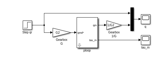
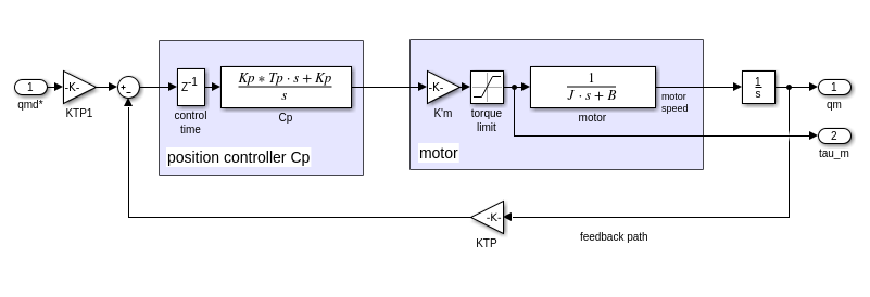
Before running the Simulink model, it is necessary to previously execute the script position_feedback_control_design.m that does the design of a PI controller, which is reproduced next:

clear
%Motor Transfer function (voltage to velocity): M(s) = Kmm / (s*Im + Bm)
Im = 581e-6 % Total inertia seen by motor of joint 2 as computed by:
            %   >> mdl_puma560
            %   >> p560_inertia_evaluation
            %   >> Jm = p560.links(2).Jm + meanB22 / p560.links(2).G^2
Bm = 817e-6 % Joint 2 viscous friction: p560.links(2).B
Kmm = 0.228 % Motor 2 torque constant from Table 9.1 page 205 Corke book

%Motor Transfer function (voltage to velocity): M(s) = Km / (s*Tm + 1)        
Tm = Im/Bm
Km = Kmm/Bm
Gpp = tf([Kmm],[Im Bm 0])

%Other motor constants:
G2 = 107.815 %Joint 2 Gear ratio: p560.links(2).G
tau_max = 0.9 %Maximum torke of motor 2 from Table 9.1 page 205 Corke book

%PI controller transfer function
Tp = 10  %chosen 10 times greater than Tm
Kp = 1 %to be adjusted
Cp = tf([Kp*Tp Kp],[1 0])

%Encoder transfer function
KTP = 1

%Open loop transfer function
L = KTP*series(Cp,Gpp)

%Root locus
%rlocus(L)
h=rlocusplot(L); 
p = getoptions(h);
p.YLim={[-2.5 2.5]};
setoptions(h,p);

%Choose the poles near -1/Tp
K = rlocfind(L)

%Adjust Kp value by multiplying by the factor found by rlocfind
Kp = K*Kp
Cp = tf([Kp*Tp Kp],[1 0])
L = KTP*series(Cp,Gpp) 
W = feedback(L,1)
[zeros,pols,k] = zpkdata(W,'v')

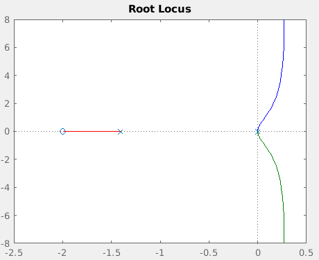
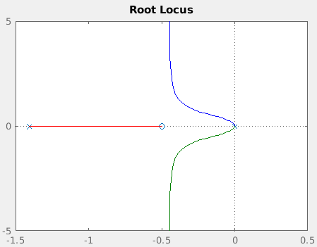
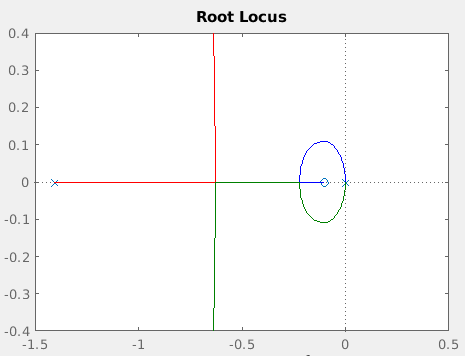
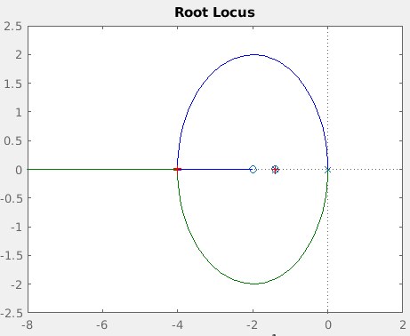
In the design script, the \(T_p\) has been set greater than \(T_m\) to assure stability, otherwise two of the root locus branches lie completely on the right-half plane, as shown in these figures for \(T_p<T_m\), \(T_p>T_m\) and \(T_p>>T_m\):

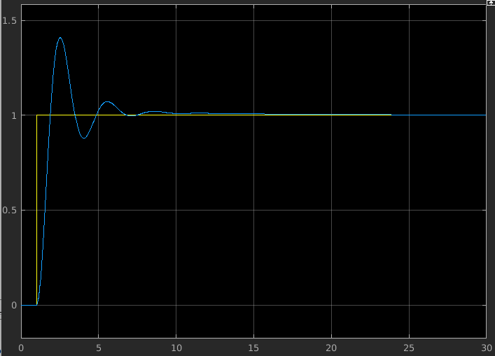
../_images/rlocusPosFeedback_SmallTp.png

../_images/rlocusPosFeedback_VeryBigTp.png

The value of \(K_p\) is set with the script by selecting the desired closed loop poles in the root locus (by means of the rlocfind function). If one pole is approximately chosen at the position of the zero (to be canceled by it), then the time response is that of a second order system with complex poles.

position_feedback_control_design

Exercise

Run the Simulink model to see the response to a step. Repeat by varying the control parameters chosen.

Position-velocity feedback control scheme

The file pos_vel_feedback_control_test.slx contains the Simulink model of the position-velocity feedback control scheme.

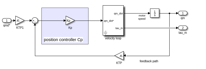
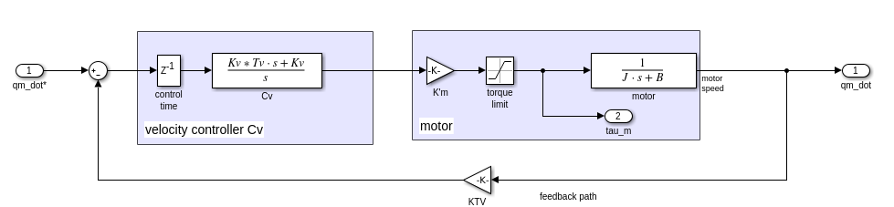
Before running the Simulink model, it is necessary to previously execute the script pos_vel_feedback_control_design.m that does the design of a PI controller for the velocity loop and a P controller for the position loop. It is reproduced next:

clear
%Motor Transfer function (voltage to velocity): M(s) = Kmm / (s*Im + Bm)
Im = 581e-6 % Total inertia seen by motor of joint 2 as computed by:
            %   >> mdl_puma560
            %   >> p560_inertia_evaluation
            %   >> Jm = p560.links(2).Jm + meanB22 / p560.links(2).G^2
Bm = 817e-6 % Joint 2 viscous friction: p560.links(2).B
Kmm = 0.228 % Motor 2 torque constant from Table 9.1 page 205 Corke book

%Motor Transfer function (voltage to velocity): M(s) = Km / (s*Tm + 1)
Tm = Im/Bm
Km = Kmm/Bm

%Other motor constants:
G2 = 107.815 %Joint 2 Gear ratio: p560.links(2).G
tau_max = 0.9 %Maximum torke of motor 2 from Table 9.1 page 205 Corke book

%P controller transfer function - position loop
Kp = 2 %Much greater values than 2 will make the torque reach its max value 

%PI controller transfer function - velocity loop
Tv = Tm %made equal to Tm, then zero of controller cancels pole of motor
Kv = 1 %to be adjusted

%Encoder transfer function
KTP = 1
%Tachometer transfer function
KTV = 1

%Open loop transfer function
P = tf(Km*Kp*Kv*[Tv 1],[Tm 1 0 0])
H = KTP*tf([KTV/(Kp*KTP) 1],1)
L = series(P,H)

%Root locus
rlocus(L)
%Choose the poles near -1/Tp
K = rlocfind(L)

%Adjust Kp value by multiplying by the factor found by rlocfind
Kv = K*Kv
P = tf(Km*Kp*Kv*[Tv 1],[Tm 1 0 0])
H = KTP*tf([KTV/(Kp*KTP) 1],1) 
W = feedback(P,H)
[zeros,pols,k] = zpkdata(W,'v')

In the design script:

The \(K_p\) has been set to 2 (this fixes the zero; greater values would easily make the maximum allowed torque to be reached),
The \(T_v\) has been set equal to \(T_m\) to cancel one pole (then a second-order system results), and
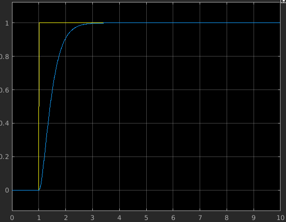
The \(K_v\) is set by selecting the desired closed loop poles in the root locus (for instance they can be selected to be real and equal).

../_images/posvelFeedback_stepResponse.png

pos_vel_feedback_control_design

Exercise

Execute the Simulink model to see the response to a step. Repeat by varying the control parameters chosen.

Effect of the gravity

The decentralized approach treats nonlinearities and coupling as disturbances to be rejected. The effect of gravity is an important part; for instance the gravity torque on joint 2 of the Puma 560 manipulator ranges from -40 to 40 N m.

To illustrate this, let’s consider as a disturbance an input equal to half the maximum gravity torque at that joint, i.e. 20 N m, both for the position feedback control scheme and for the position-velocity position control scheme:

The file position_feedback_control_with_D_test.slx. contains the Simulink model of the position feedback control scheme that includes the disturbance term due to gravity.

The file pos_vel_feedback_control_with_D_test.slx. contains the Simulink model of the position-velocity feedback control scheme that includes the disturbance term due to gravity.

Exercise

Execute both models (with both alternative inputs offered) to verify that the control schemes are able to cope with this disturbance. .

Decentralized feed forward compensation

For tracking problems, the behavior of the system can be improved if feed-forward schemes are used:

The file position_feedback_control_with_FF_test.slx. contains the Simulink model of the position feedback control scheme that includes the feed-forward terms.

The file pos_vel_feedback_control_with_FF_test.slx. contains the Simulink model of the position-velocity feedback control scheme that includes the feed-forward terms.

Exercise

Execute both models to verify the improvements in the performance in the problem of tracking a sinusoidal input.

Centralized control schemes

PD control with gravity compensation in the joint space

The file PD_gravity_joint_space.slx. contains the Simulink model of the PD control with gravity compensation in the joint space for the PUMA 560 robot, and the script centralized_control_design.m the KP and KD control parameters.

Run the model to verify the performance (be patient; the simulation is slow):

mdl_puma560
centralized_control_design
open PD_gravity_joint_space

Exercise

Verify that the torques are under its limits. Monitorize the error, and check that the derivative term actually accelerates the convergence rate.

Inverse dynamic control in the joint space

The file inverse_dynamic_control.slx. contains the Simulink model of the inverse dynamic control scheme in the joint space for the PUMA 560 robot, and the script centralized_control_design.m the KP and KD control parameters.

mdl_puma560
centralized_control_design
open inverse_dynamic_control

Exercise

Check that the Simulink model effectively implements the inverse dynamic model. Verify that the output tracks the input desired trajectory. Repeat for different values of the control parameters. You can also try shorter durations of the input trajectory (tmax).

EXERCISE (Deliverable)

Consider a three-link planar arm with the following properties:

It works on the xy-plane (with the gravity in the -y direction)
All the links are equal.
The geometry of the links is cylindrical (length equal to the length of link 2 of the Puma 560 manipulator and the radius is 0.05 m).
The dynamic properties of the links are equal to those of link 2 of the Puma 560 manipulator, except the motor inertia that is set to zero and the inertia and center of mass that have to be set according to the cylindrical shape.
The torque limits is 400.

Obtain the dynamic model (inertia and Coriolis matrices and the friction and gravitational terms) and check the correctness by also modeling it using the Robotics Toolbox. You can make use of all the scripts provided in the Dynamics tutorial.
Implement an inverse dynamic_control scheme without using the Robotics Toolbox. You can use the Simulink blocks Interpreted MATLAB Fcn and Matrix Multilpy, as done in the demo_eval_Bqdd.slx model.
Make a variant of the previous control scheme, where only the dominant terms are computed in order to lighten the computational load. Verify that the performance is only slightly affected.