Decentralized motion control

Based on Section 8.3 of Robotics: Modelling, Planning and Control.

Link to the practical session on Decentralized control schemes

Idea and General schema

This control scheme considers the manipulator as a set of \(n\) independent systems, each one controlled as a SISO system, and the couplings are treated as disturbances.

Let’s rewrite the dynamics of the manipulator in terms of \(\boldsymbol{q}_m\) and \(\boldsymbol{\tau}_m\):

\[\boldsymbol{q} = k_r^{-1} \boldsymbol{q}_m\]

\[\boldsymbol{\tau} = k_r \boldsymbol{\tau}_m\]

Then, \(B(\boldsymbol{q}) \ddot{\boldsymbol{q}} + C(\boldsymbol{q}, \dot{\boldsymbol{q}}) \dot{\boldsymbol{q}} + F_v \dot{\boldsymbol{q}} + \boldsymbol{g}(\boldsymbol{q}) = \boldsymbol{\tau}\) becomes:

\[k_r^{-1} B(\boldsymbol{q}) k_r^{-1} \ddot{\boldsymbol{q}}_m + k_r^{-1} C(\boldsymbol{q}, \dot{\boldsymbol{q}}) k_r^{-1} \dot{\boldsymbol{q}}_m + k_r^{-1} F_v k_r^{-1} \dot{\boldsymbol{q}}_m + k_r^{-1} \boldsymbol{g}(\boldsymbol{q}) = \boldsymbol{\tau}_m\]

That can be rewritten as:

\[k_r^{-1} \boldsymbol B k_r^{-1} \ddot{\boldsymbol{q}}_m + F_m \dot{\boldsymbol{q}} = \boldsymbol{\tau}_m - \boldsymbol{d}\]

where:

\[B(\boldsymbol{q}) = \boldsymbol{B} + \Delta B(\boldsymbol{q})\]

\[\boldsymbol{B} \text{ is a diagonal matrix; its constant elements represent the average inertia at each joint.}\]

\[\Delta B(\boldsymbol{q}) \text{ contains the configuration-dependent terms (function of sine and cosine for revolute joints).}\]

\[F_m = k_r^{-1} F_v k_r^{-1}\]

\[\boldsymbol{d} = k_r^{-1} \Delta B(\boldsymbol{q}) k_r^{-1} \ddot{\boldsymbol{q}}_m + k_r^{-1} C(\boldsymbol{q}, \dot{\boldsymbol{q}}) k_r^{-1} \dot{\boldsymbol{q}}_m + k_r^{-1} \boldsymbol{g}(\boldsymbol{q})\]

\[\boldsymbol{d} \text{ contains all the coupling terms and will be considered as a disturbance.}\]

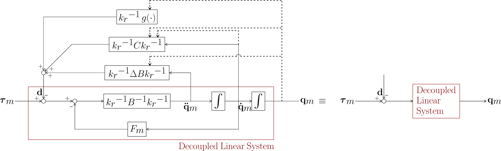
Now, in order to control each joint of the decoupled linear system, different SISO control schemes are proposed:

1. Position feedback control scheme

2. Position/velocity feedback control scheme

3. Position/velocity/acceleration feedback control scheme

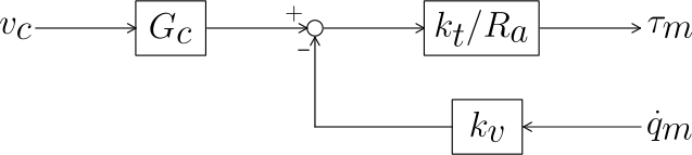
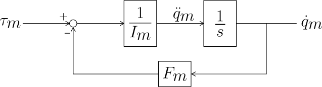
Let’s first derive the transfer function of the motor and the velocity-controlled drive.

Drive

\[\tau_m = k_t i_a\]

\[v_a = R_a i_a + k_v \dot{q}_m\]

\[v_a = G_c v_c\]

Motor

\[I_m \ddot{q}_m = \tau_m - F_m \dot{q}_m\]

Then, the ensemble Drive+Motor is the following, where a load reaction torque \(D\) has been added:

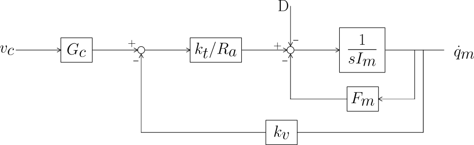
This block scheme can be simplified to:

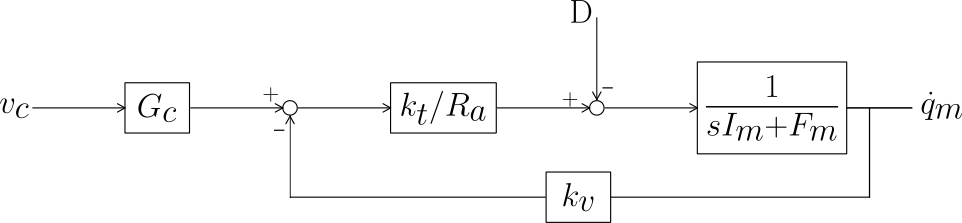
Then:

\[M(s) = \frac{\frac{k_t}{R_a} \frac{1}{s I_m + F_m}}{1 + \frac{k_t}{R_a} k_v \frac{1}{s I_m + F_m}} = \frac{\frac{k_t}{R_a}}{s I_m + \underbrace{F_m + \frac{k_t k_v}{R_a}}_{ F_m \ll \frac{k_t k_v}{R_a}}} = \frac{1/k_v}{s \frac{I_m R_a}{k_t k_v} + 1} = \frac{k_m}{T_m s + 1}\]

where:

\[k_m = \frac{1}{k_v}, \quad T_m = \frac{I_m R_a}{k_t k_v}\]

Position feedback scheme

The gain \(G_c\) appearing in the previous schema is absorbed here by \(C_P(s)\).

\[k_{TP} \text{ : potentiometer / encoder gain}\]

\[C_P(s) = K_P \frac{1 + s T_P}{s} \quad \text{PI controller}\]

\[G(s) = \frac{k_m}{s (1 + s T_m)}\]

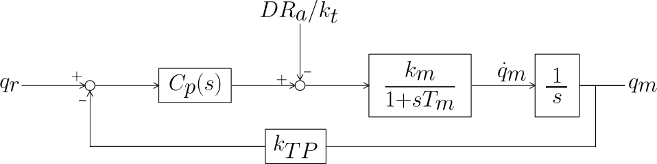
The transfer function of the forward path is:

\[P(s) = C_P(s)G(s) = \frac{K_P k_m (1 + s T_P)}{s^2 (1 + s T_m)},\]

while that of the return path is:

\[H(s) = k_{TP}\]

Finally, the closed-loop transfer function is:

\[W(s) = \frac{P(s)}{1 + P(s) H(s)} = \frac{\left(\frac{1}{k_{TP}}\right)(1 + s T_P)}{\left(1 + \frac{2 \xi}{\omega_n} s + \frac{s^2}{\omega_n^2}\right)(1 + s \tau)}\]

Three different root loci are possible according to the values of \(T_m\), \(T_P\):

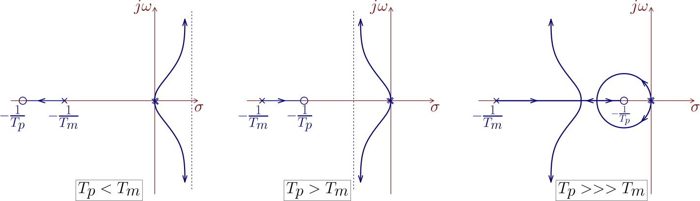
Considering the third case:

• Pole cancellation:

  • The real pole of \(W(s)\) is \(\frac{1}{\tau} \approx \frac{1}{T_P}\) for high values of \(K_p\). Then, its effect tends to be cancelled by the zero of \(W(s)\).

• Disturbance rejection:

  • Considering the transfer function between the disturbance and the output \(W_D = \frac{-k_m}{T_m s^3 + s^2 + K_p k_m k_{TP} T_P s + k_m k_p k_{TP}}\)

  • Then, \(\lim_{s \to 0} W_D = -\frac{1}{k_{TP} K_P}\), i.e. the rejection ratio is \(X_R = K_P k_{TP}\)

• System response:

  • The value of \(K_P\) determines the poles and therefore the response of the system.

  • For high values of \(K_P\), desired for disturbance rejection, too small damping ratios may result ⇒ trade-off!

Position and velocity feedback scheme

\[k_{TV} \text{: tachometer gain}\]

\[k_{TP} \text{: encoder gain}\]

\[C_P(s) = K_P \quad\quad\quad\quad\quad \text{ P controller}\]

\[C_V(s) = K_V \frac{1 + s T_V}{s} \quad \text{ PI controller}\]

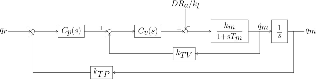
Now the transfer functions of the forward and return paths are:

\[\begin{split}\left. \begin{aligned} P(s) &= \frac{k_m K_P K_V (1 + s T_V)}{s^2 (1 + s T_m)} \\ H(s) &= k_{TP} \left( {1 + s \frac{k_{TV}}{K_P k_{TP}}} \right) \end{aligned} \right\} \quad \quad L(s) = P(s) H(s) \quad \text{(open loop transfer function)}\end{split}\]

If we choose \(T_V = T_m\), then the zero of the controller cancels the pole of the motor, and the root locus results:

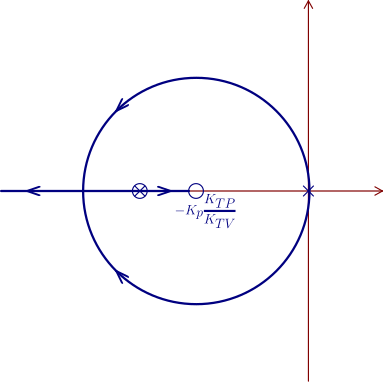
Root locus parameterized by \(k_m K_P K_V\)

Now we can observe that:

• Large values of \(K_P\) bring the branches towards large negative values (because it moves the zero to the left), therefore fast responses are achieved.

• \(K_V\) can be used to obtain the actual values of the closed loop poles.

• In fact, with \(K_P\) and \(K_V\) we can fix the two poles of the closed loop system for a given desired specification of \(\xi\) and \(\omega_n\).

• The disturbance ratio is now \(X_R = K_P k_{TP} K_V\)

\[\left( \lim_{s \to 0} W_D = -\frac{1}{K_P k_{TP} K_V} \right)\]

Also, in general, the fulfillment of the specifications using high values of the controller constants may produce some problems due to:

• Unmodelled dynamics, like electronic dynamics, elastic dynamics, filter dynamics…

• Saturation in velocity, acceleration, motor voltage.

• Implementation in discrete time with a finite sampling rate.