Visual servoing

The visual servoing problem

Objective: To ensure that the end-effector of the manipulator reaches and keeps a desired pose w.r.t. an observed object.

Objects are observed with a camera, and image processing techniques, like image segmentation and interpretation, are used to extract the image feature parameters.

The stated problem can be solved in two ways:

• The look-and-move approach uses visual measurements in open-loop. Therefore, it is sensitive to uncertainties like the possible poor position accuracy of the manipulator or the uncertainties in the actual location of the objects.

• The visual-servoing approach proposes the use of visual measurements in closed-loop, i.e., visual measurements are continuously fed back to the controller to compute the appropriate command to achieve the goal.

As a difference with other feedback control schemes, visual-servoing has controlled variables not directly measured by a sensor, but obtained by a computationally expensive process.

The visual servoing problem depends on:

1. The position of the camera

• Eye-to-hand: camera fixed w.r.t. the world. It has fixed accuracy but problems of occlusion.

• Eye-in-hand: camera held by the gripper. It solves occlusion problems but has variable accuracy as the manipulator approaches the objects. (Although this is not that relevant when near the object)

2. Number of cameras:

• One camera: simple; constrained to 2D vision

• Two cameras: allow the use of the stereo vision and the obtaining of 3D info that may help the pose estimation algorithms.

3. Object motion:

• Fixed object: Regulation problem.

• Moving object: Tracking problem. More complex due to the computational cost of visual-servoing loops.

4. Space where the control is done:

• Operational space: Requires the computation of the pose of the object and a position-based visual servoing scheme.

- Advantages: A desired time response of the end effector motion can be obtained by selecting the appropriate control parameters. - Disadvantages: It requires the knowledge of the object, it is sensitive to camera calibration, and no direct control of the image parameters may lead the object to be outside the field of view.

• Image space: Now the control action is computed on the basis of the error between image feature parameters at the current configuration and at the desired one.

- Advantages: The real time estimation of the object pose is not needed, and the object is always kept inside the camera field of view. - Disadvantages: Non-linearities in the mapping between the object features and the corresponding image parameters may lead to singularities in the manipulator motion.

Position-based visual servoing

We will consider the position-based visual-servoing problem considering a single hand-held camera and fixed objects.

An important part of the position-based visual servoing loop is the estimation of the end-effector pose. This can be done using:

• Analytical methods: They are based on the correspondance of a certain number of points.

With the knowledge of some points on the object :math:`P_i`, :math:`i = 1 \dots n` defined by the vector :math:`\boldsymbol{r_i}^0`, and the corresponding image features on the (virtual) image plane :math:`\boldsymbol S_i`, a system of equations can be set whose unknowns are the values of the transformation :math:`{T_0}^c` that locates the object w.r.t. the camera frame.

• Iterative numerical algorithms: They are based on the integration of the linear mapping between the camera velocity in the operational space and the time-derivative of the feature parameters in the image plane.

Output: The output of the pose estimation is the homogeneous transformation \({T_0}^c\) and \(\boldsymbol{x}_{c,o} = \begin{bmatrix}\boldsymbol{\theta}^c_{c,o} \\ \boldsymbol{\phi}_{c,o} \end{bmatrix}\) a vector of minimum number of coordinates, with \(\boldsymbol{\theta}^c_{c,o}\) expressing the position and \(\boldsymbol{\phi}_{c,o}\) the orientation using Euler angles.

PD control with gravity compensation

The PD control with gravity compensation scheme in the operational space, with the same error definition used in the force control scheme, can be used together with a pose estimation procedure.

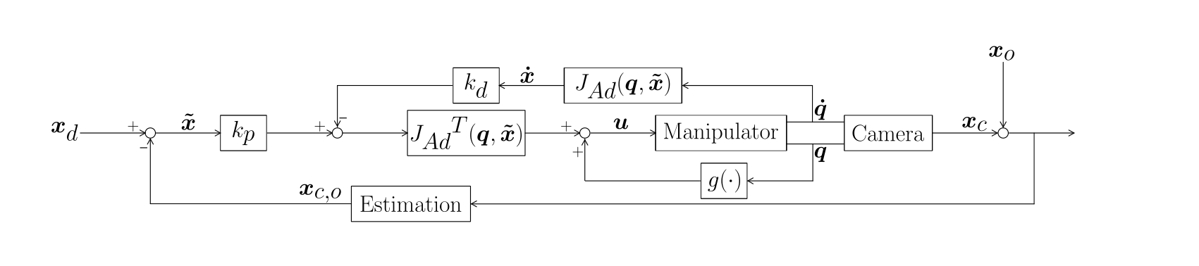
• Set point: \(T^d_o\), a desired transformation between the object and the camera located at the end-effector.

\(T^d_o\) is expressed in the schema as \(\boldsymbol{x}_d = \begin{bmatrix} \boldsymbol{\theta}^d_{d,o}, \boldsymbol{\phi}_{d,o} \end{bmatrix}^T\)

• Measurement: \(T^c_o\), expressed as \(\boldsymbol{x}_{c,o}\)

• Error: The difference between \(T^d_o\) and \(T^c_o\), i.e.,

\[\begin{split}T^d_e = T^d_o (T^c_o)^{-1} = \begin{bmatrix} R^d_c & \boldsymbol{\theta}^d_{d,c} \\ \boldsymbol{0}^T & 1 \end{bmatrix}\end{split}\]

\[\begin{split}\tilde{\boldsymbol{x}} = - \begin{bmatrix} \boldsymbol{\theta}^d_{d,c} \\ \boldsymbol{\phi}_{d,c} \end{bmatrix} , \quad \text{with } \boldsymbol{\phi}_{d,c} \text{ the Euler angles corresponding to } R^d_c\end{split}\]

• The control law is:

\[\boldsymbol{u} = \boldsymbol{g}(\boldsymbol{q}) + J^T_{Ad}(\boldsymbol{q}, \tilde{\boldsymbol{x}}) \left[ k_p \tilde{\boldsymbol{x}} - k_d J_{Ad}(\boldsymbol{q}, \tilde{\boldsymbol{x}}) \boldsymbol{\dot{q}} \right]\]

with

\[\begin{split}J_{Ad}(\boldsymbol{q}, \tilde{\boldsymbol{x}}) = T_A^{-1}(\boldsymbol{\phi}_{d,c}) \begin{bmatrix} R_d^T & 0 \\ 0 & R_d^T \end{bmatrix} J(\boldsymbol{q})\end{split}\]

with \(k_p\) and \(k_d\) positive definite, this control brings the error asymptotically to zero.

This schema was used in force control because it allowed a direct and decoupled active compliant behaviour, described by matrix \(k_p\), defined w.r.t. a reference frame related to the task.

Now, this schema is used because the most natural reference frame to work with is that of the camera.

The steps of the control procedure are the following:

1. Compute \(T^c_o\) using a pose estimation procedure.

2. Compute the transform between the desired and the current pose:

\[\begin{split}T^d_c = T^d_o (T^c_o)^{-1} = \begin{bmatrix} R^d_c & \boldsymbol{\theta}^d_{c,d} \\ \boldsymbol{0}^T & 1 \end{bmatrix}\end{split}\]

3. Compute the error:

\[\begin{split}\tilde{\boldsymbol{x}} = \begin{bmatrix} \boldsymbol{\theta}^d_{c,d} \\ \boldsymbol{\phi}_{c,d} \end{bmatrix}\end{split}\]

with \(\boldsymbol{\phi}_{c,d}\) the XYZ Euler angles associated to \(R^d_c\).

Note

\(\tilde{\boldsymbol{x}}\) is not obtained directly from \(\boldsymbol{x}_d\) and \(\boldsymbol{x}_{c,o}\).

4. Compute the analytical Jacobian \(J_{Ad}(\boldsymbol{q}, \tilde{\boldsymbol{x}})\)

5. Apply the control law \(\boldsymbol{u}\):

\[\boldsymbol{u} = g(\boldsymbol{q}) + J^T_{Ad}(\boldsymbol{q}, \tilde{\boldsymbol{x}}) \left[ k_p \tilde{\boldsymbol{x}} - k_d J_{Ad}(\boldsymbol{q}, \tilde{\boldsymbol{x}}) \boldsymbol{\dot{q}} \right]\]

This is a computationally costly procedure, which requires a low sampling frequency (large sampling times). As a consequence:

• Low gains are required to guarantee stability.

• The performance in terms of disturbance rejection is low.

• The performance in terms of speed of convergence is low.

Resolved velocity control

To overcome the above mentioned problems, an alternative is:

1. To consider the manipulator equipped with a high-gain motion controller, i.e., consider the manipulator as an ideal positioning device \(\boldsymbol{q}(t) \approx \boldsymbol{q}_r(t)\), where \(\boldsymbol{q}_r(t)\) is the reference trajectory.

2. To use the visual servoing to compute \(\boldsymbol{q}_r(t)\).

This way, visual servoing is achieved by computing \(\boldsymbol{q}_r(t)\) on the basis of visual measurements and using the analytical Jacobian \(J_{Ad}(\boldsymbol{q}, \tilde{\boldsymbol{x}})\).

• The error is, as before \(\tilde{\boldsymbol{x}} = - \begin{bmatrix} \boldsymbol{\theta}^d_{d,c} \\ \boldsymbol{\phi}_{d,c} \end{bmatrix}\).

• The time derivative of the error (as demonstrated in the force control section) is \(\dot{\tilde{\boldsymbol{x}}} = -J_{Ad}(\boldsymbol{q}, \tilde{\boldsymbol{x}}) \, \boldsymbol{\dot{q}}\).

• If we chose the joint space reference velocity \(\boldsymbol{\dot{q}}_r(t)\) as \(\boldsymbol{\dot{q}}_r = J_{Ad}^{-1}(\boldsymbol{q}, \tilde{\boldsymbol{x}}) \, k \, \tilde{\boldsymbol{x}}\).

Then, since \(\boldsymbol{q}(t) \approx \boldsymbol{q}_r(t)\) we have that:

\[\dot{\tilde{\boldsymbol{x}}} = -J_{Ad}(\boldsymbol{q}, \tilde{\boldsymbol{x}}) \left[ J^{-1}_{Ad}(\boldsymbol{q}, \tilde{\boldsymbol{x}}) \, k \, \tilde{\boldsymbol{x}} \right]\]

\[\dot{\tilde{\boldsymbol{x}}} = -k \tilde{\boldsymbol{x}}\]

\[\boxed{ \dot{\tilde{\boldsymbol{x}}} + k \tilde{\boldsymbol{x}} = 0}\]

i.e., for \(k\) positive definite, the error \(\tilde{\boldsymbol{x}}\) is brought asymptotically to zero, with a convergence of exponential type and speed depending on the eigenvalues of \(k\).

This schema is called resolved-velocity control in the operational space, because it is based on the computation of \(\boldsymbol{\dot q}\) from the operational space error.

The trajectory \(\boldsymbol{q}_r(t)\) is computed from \(\boldsymbol{\dot{q}}(t)\) by a simple integration.

• If \(k\) is a diagonal matrix with the same signs for the translational part, the origin of the camera frame follows the line segment connecting the initial position to the desired one.

• The orientation trajectory, however, depends on the particular choice of Euler angles used to define the orientation error.

The possibility to know in advance the trajectory of the camera is important because, during the motion, the object may exit from the camera field of view, making its visual measurements unavailable.