Centralized motion control

Based on Sections 8.5 and 8.6 of Robotics: Modelling, Planning and Control.

Link to the practical session on Centralized control schemes

Introductory comments

• If large speeds are required and/or direct-drive actuation is used, the non-linear coupling terms have a great influence.

• It is advisable to design control schemes that take advantage of a detailed knowledge of the manipulator dynamics to compensate for the non-linear couplings, rather than try to reduce their effect, i.e. to use centralised control schemes.

• The computed-torque FF compensation presented in the previous section worked in this line, but it was computed on the desired trajectory; what is proposed now is to use the dynamic model in closed loop.

• Two control schemes will be discussed here:

  1. PD control with gravity compensation in the joint space and in operational space.

  2. Inverse dynamic control in the joint space.

PD control with gravity compensation in the joint space

Consider a regulation problem where a fixed configuration \(\boldsymbol{q}_d\) is desired, then the error is \(\tilde{\boldsymbol{q}} = \boldsymbol{q}_d - \boldsymbol{q}\) and the system state can be defined as \([\tilde{\boldsymbol{q}}^T, \dot{\boldsymbol{q}}^T]\).

Question: Which control law \(\boldsymbol{u}\) can bring the manipulator (with dynamics \(B(\boldsymbol{q}) \ddot{\boldsymbol{q}} + C(\boldsymbol{q}, \dot{\boldsymbol{q}}) \dot{\boldsymbol{q}} + F \dot{\boldsymbol{q}} + \boldsymbol{g}(\boldsymbol{q}) = \boldsymbol{u}\)) towards \(\boldsymbol{q}_d\) in an asymptotically stable manner?

Using Lyapunov direct method

The Lyapunov direct method can be used to determine such law.

• If a Lyapunov function \(V(\tilde{\boldsymbol{q}}, \dot{\boldsymbol{q}})\) is found such that \(\dot{V}(\tilde{\boldsymbol{q}}, \dot{\boldsymbol{q}}) < 0\) along all the trajectories, then the system is asymptotically stable.

• \(V(\tilde{\boldsymbol{q}}, \dot{\boldsymbol{q}})\) is usually set as a function of the system energy.

Let’s consider the following positive definite quadratic form:

\[V(\tilde{\boldsymbol{q}}, \dot{\boldsymbol{q}}) = \frac{1}{2} \dot{\boldsymbol{q}}^T B(\boldsymbol{q}) \dot{\boldsymbol{q}} + \frac{1}{2} \tilde{\boldsymbol{q}}^T\, K_P\, \tilde{\boldsymbol{q}} > 0 \quad \forall \boldsymbol{\dot q}, \tilde{\boldsymbol{q}} \ne 0\]

with \(K_P\) a \((n \times n)\) matrix, positive definite.

Differentiating w.r.t. time and recalling that \(\boldsymbol{q}_d\) is constant (i.e., \(\dot{\tilde{\boldsymbol{q}}} = \dot{\boldsymbol{q}}_d - \dot{\boldsymbol{q}} = -\dot{\boldsymbol{q}}\)):

\[\dot{V}(\tilde{\boldsymbol{q}}, \dot{\boldsymbol{q}}) = \frac{1}{2} \dot{\boldsymbol{q}}^T (\dot{B}(\boldsymbol{q}) \dot{\boldsymbol{q}} + \underbrace{B(\boldsymbol{q}) \ddot{\boldsymbol{q}}) + \frac{1}{2} \ddot{\boldsymbol{q}}^T B(\boldsymbol{q}) \dot{\boldsymbol{q}}}_{\boldsymbol{\dot q}^T B(\boldsymbol q) \boldsymbol{\ddot q}} + \frac{1}{2} \dot{\tilde{\boldsymbol{q}}}^T\, K_P \,\tilde{\boldsymbol{q}} + \frac{1}{2} \tilde{\boldsymbol{q}}^T\, K_P\, \dot{\tilde{\boldsymbol{q}}}\]

\[\dot{V}(\tilde{\boldsymbol{q}}, \dot{\boldsymbol{q}}) = \frac{1}{2} \dot{\boldsymbol{q}}^T \dot{B}(\boldsymbol{q}) \dot{\boldsymbol{q}} + \dot{\boldsymbol{q}}^T \underbrace{B(\boldsymbol{q}) \ddot{\boldsymbol{q}}} - \dot{\boldsymbol{q}}^T K_P \tilde{\boldsymbol{q}}\]

From the system dynamics, \(B(\boldsymbol{q}) \ddot{\boldsymbol{q}} = \boldsymbol{u} - C(\boldsymbol{q}, \dot{\boldsymbol{q}}) \dot{\boldsymbol{q}} - F \dot{\boldsymbol{q}} - \boldsymbol{g}(\boldsymbol{q})\), then:

\[\dot{V}(\tilde{\boldsymbol{q}}, \dot{\boldsymbol{q}}) = \frac{1}{2} \dot{\boldsymbol{q}}^T \dot{B}(\boldsymbol{q}) \dot{\boldsymbol{q}} + \dot{\boldsymbol{q}}^T \left[ \boldsymbol{u} - C(\boldsymbol{q}, \dot{\boldsymbol{q}}) \dot{\boldsymbol{q}} - F \dot{\boldsymbol{q}} - \boldsymbol{g}(\boldsymbol{q}) \right] - \dot{\boldsymbol{q}}^T K_P \tilde{\boldsymbol{q}}\]

\[\dot{V}(\tilde{\boldsymbol{q}}, \dot{\boldsymbol{q}}) = \frac{1}{2} \dot{\boldsymbol{q}}^T \left[ \dot{B} - 2C \right] \dot{\boldsymbol{q}} - \dot{\boldsymbol{q}}^T F \dot{\boldsymbol{q}} + \dot{\boldsymbol{q}}^T \left[ \boldsymbol{u} - \boldsymbol{g}(\boldsymbol{q}) - K_P \tilde{\boldsymbol{q}} \right]\]

Note

\(N = \dot{B} - 2C\) is a skew symmetric matrix (see properties). Then \(\dot{\boldsymbol{q}}^T N \dot{\boldsymbol{q}} = 0\)

Considering this:

\[\dot{V}(\tilde{\boldsymbol{q}}, \dot{\boldsymbol{q}}) = - \dot{\boldsymbol{q}}^T F \dot{\boldsymbol{q}} + \dot{\boldsymbol{q}}^T \underbrace{\left[ \boldsymbol{u} - \boldsymbol{g}(\boldsymbol{q}) - K_P \tilde{\boldsymbol{q}} \right]}\]

In order to achieve \(\dot{V}(\boldsymbol{q}, \dot{\boldsymbol{q}}) < 0\), this term can be made zero by choosing the following control law:

\[\boldsymbol{u} = \boldsymbol{g}(\boldsymbol{q}) + K_P \tilde{\boldsymbol{q}}\]

Therefore:

\[\dot{V}(\tilde{\boldsymbol{q}}, \dot{\boldsymbol{q}}) = - \dot{\boldsymbol{q}}^T F \dot{\boldsymbol{q}} < 0 \Rightarrow \text{The system is asymptotically stable.}\]

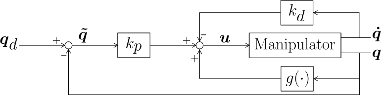
The chosen control law:

• has gravity compensation.

• has a proportional term.

Improving the performance

Convergence can be accelerated if a derivative term is added, described by a positive definite matrix \(K_D\):

\[\boxed{ \boldsymbol{u} = \boldsymbol{g}(\boldsymbol{q}) + K_P \tilde{\boldsymbol{q}} - K_D \dot{\boldsymbol{q}}}\]

This results in a PD controller with gravity compensation.

Now, the derivative of \(V(\boldsymbol{q}, \dot{\boldsymbol{q}})\) is:

\[\dot{V}(\tilde{\boldsymbol{q}}, \dot{\boldsymbol{q}}) = -\dot{\boldsymbol{q}}^T (F + K_D) \dot{\boldsymbol{q}} < 0\]

According to this, \(V\) decreases for all the system trajectories, as long as \(\dot{\boldsymbol{q}} \ne 0\).

The dynamics of the system with the PD controller is:

\[B(\boldsymbol{q}) \ddot{\boldsymbol{q}} + C(\boldsymbol{q}, \dot{\boldsymbol{q}}) \dot{\boldsymbol{q}} + F\dot{\boldsymbol{q}} + \boldsymbol{g}(\boldsymbol{q}) = \underbrace{\boldsymbol{g}(\boldsymbol{q}) + K_P \tilde{\boldsymbol{q}} - K_D \dot{\boldsymbol{q}}}_{\boldsymbol u}\]

At the equilibrium point we have that: \(\dot{\boldsymbol{q}} = \ddot{\boldsymbol{q}} = 0\), which makes the dynamics simplify to:

\[K_P \tilde{\boldsymbol{q}} = 0\]

i.e., the desired configuration is attained:

\[\tilde{\boldsymbol{q}} = \boldsymbol{q}_d - \boldsymbol{q} = 0\]

Any manipulator equilibrium posture is globally asymptotically stable under a PD controller with gravity compensation (using \(K_P\) and \(K_D\) positive definite matrices).

PD control with gravity compensation in the operational space

Consider now a regulation problem where a fixed end-effector pose \(\boldsymbol{x}_d\) is desired, then the error is \(\tilde{x} = \boldsymbol{x}_d - \boldsymbol{x}_e\) and the system state can be defined as \([\tilde{\boldsymbol{x}}^T, \dot{\boldsymbol{q}}^T]\).

Question: Which control law \(\boldsymbol{u}\) can bring the manipulator (with dynamics \(B(\boldsymbol{q}) \ddot{\boldsymbol{q}} + C(\boldsymbol{q}, \dot{\boldsymbol{q}}) \dot{\boldsymbol{q}} + F \dot{\boldsymbol{q}} + \boldsymbol{g}(\boldsymbol{q}) = \boldsymbol{u}\)) towards \(\boldsymbol{x}_d\) in an asymptotically stable manner?

Using Lyapunov direct method

Let’s consider the following positive definite quadratic form:

\[V(\boldsymbol{\dot q}, \tilde{\boldsymbol x}) = \frac{1}{2} \dot{\boldsymbol{q}}^T B(\boldsymbol{q}) \dot{\boldsymbol{q}} + \frac{1}{2} \tilde{\boldsymbol x}^T K_P \tilde{\boldsymbol x} > 0 \quad \forall \boldsymbol{\dot q}, \tilde{\boldsymbol x} \ne 0\]

with \(K_P\) a \((n \times n)\) positive definite matrix.

Its time derivative is (similarly as done before):

\[\dot{V}(\boldsymbol{\dot q}, \tilde{\boldsymbol x}) = \dot{\boldsymbol{q}}^T B(\boldsymbol{q}) \ddot{\boldsymbol{q}} + \frac{1}{2} \dot{\boldsymbol{q}}^T \dot{B}(\boldsymbol{q}) \dot{\boldsymbol{q}} + \dot{\tilde{\boldsymbol x}}^T K_P {\tilde{\boldsymbol x}}\]

Since a constant pose is desired, we have that \(\dot{\tilde{\boldsymbol x}} = \dot{\boldsymbol{x}}_d - \dot{\boldsymbol{x}}_e = -\dot{\boldsymbol{x}}_e = -J_A(\boldsymbol{q}) \dot{\boldsymbol{q}}\)

Then:

\[\dot{V}(\boldsymbol{\dot q}, \tilde{\boldsymbol x}) = \dot{\boldsymbol{q}}^T \underbrace{B(\boldsymbol{q}) \ddot{\boldsymbol{q}}} + \frac{1}{2} \dot{\boldsymbol{q}}^T \dot{B}(\boldsymbol{q}) \dot{\boldsymbol{q}} - \dot{\boldsymbol{q}}^T J_A^T(\boldsymbol{q}) K_P \tilde{\boldsymbol x}\]

From the system dynamics, \(B(\boldsymbol{q}) \ddot{\boldsymbol{q}} = \boldsymbol{u} - C(\boldsymbol{q}, \dot{\boldsymbol{q}}) \dot{\boldsymbol{q}} - F \dot{\boldsymbol{q}} - \boldsymbol{g}(\boldsymbol{q})\) then:

\[\dot{V}(\boldsymbol{\dot q}, \tilde{\boldsymbol x}) = \dot{\boldsymbol{q}}^T \left[\boldsymbol{u} - C(\boldsymbol{q}, \dot{\boldsymbol{q}}) \dot{\boldsymbol{q}} - F \dot{\boldsymbol{q}} - \boldsymbol{g}(\boldsymbol{q}) \right] + \frac{1}{2} \dot{\boldsymbol{q}}^T \dot{B}(\boldsymbol{q}) \dot{\boldsymbol{q}} - \dot{\boldsymbol{q}}^T J_A^T(\boldsymbol{q}) K_P \tilde{\boldsymbol x}\]

\[\dot{V}(\boldsymbol{\dot q}, \tilde{\boldsymbol x}) = -\dot{\boldsymbol{q}}^T F \dot{\boldsymbol{q}} + \dot{\boldsymbol{q}}^T \underbrace{\left[\boldsymbol{u} - \boldsymbol{g}(\boldsymbol{q}) - J_A^T(\boldsymbol{q}) K_P \tilde{x} \right]} + \frac{1}{2} \underbrace{\dot{\boldsymbol{q}}^T [\dot{B} - 2C] \dot{\boldsymbol{q}}}_{= 0}\]

This term can be set to zero by choosing a control law: \(\,\,\boldsymbol{u} = \boldsymbol{g}(\boldsymbol{q}) + J_A^T(\boldsymbol{q}) K_P \tilde{\boldsymbol x}\)

Then:

\[\dot{V}(\boldsymbol{\dot q}, \tilde{\boldsymbol x}) = -\dot{\boldsymbol{q}}^T F \dot{\boldsymbol{q}} < 0 \Rightarrow \text{The system is asymptotically stable}\]

As before, the control law:

• has gravity compensation.

• has a proportional term.

Improving the performance

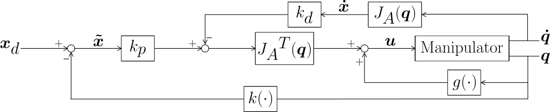
As before, convergence can be accelerated by adding a derivative term, described by a positive definite matrix \(K_D\):

\[\boxed{ \boldsymbol{u} = \boldsymbol{g}(\boldsymbol{q}) + J_A^T(\boldsymbol{q}) K_P \tilde{\boldsymbol x} - J_A^T(\boldsymbol{q}) K_D J_A(\boldsymbol{q}) \dot{\boldsymbol{q}}}\]

This results in a PD controller with gravity compensation in the operational space.

Now the derivative of \(V\) is:

\[\dot{V}(\boldsymbol{\dot q}, \tilde{\boldsymbol x}) = -\dot{\boldsymbol{q}}^T \left(F + J_A^T(\boldsymbol{q}) K_D J_A^T(\boldsymbol{q}) \right) \dot{\boldsymbol{q}} < 0\]

According to this, \(V\) decreases for all system trajectories as long as \(\dot{\boldsymbol{q}} \ne 0\).

The dynamics of the system with PD controller is:

\[B(\boldsymbol{q}) \ddot{\boldsymbol{q}} + C(\boldsymbol{q}, \dot{\boldsymbol{q}}) \dot{\boldsymbol{q}} + F \dot{\boldsymbol{q}} + \boldsymbol g(\boldsymbol{q}) = \boldsymbol{g}(\boldsymbol{q}) + J_A^T(\boldsymbol{q}) K_P \tilde{\boldsymbol x} - \underbrace{J_A^T(\boldsymbol{q}) K_D J_A^T(\boldsymbol{q}) \dot{\boldsymbol{q}}}_{\boldsymbol u}\]

At the equilibrium point, we have \(\dot{\boldsymbol{q}} = \boldsymbol{\ddot q} = 0\), and this simplifies to:

\[J_A^T(\boldsymbol{q}) K_P \tilde{\boldsymbol x} = 0\]

which means that the desired pose is achieved:

\[\tilde{\boldsymbol x} = \boldsymbol x_d - \boldsymbol x_e = 0\]

Note

Sometimes \(\boldsymbol x_e\) and \(\boldsymbol{\dot x}_e\) are directly measured and the blocks \(k(\cdot)\) and \(J_A(\boldsymbol{q})\) in the block scheme are not needed.

Inverse dynamic control in the joint space

Consider now the tracking problem where the robot has to follow a desired trajectory described by \(\boldsymbol{q}_d(t), \dot{\boldsymbol{q}}_d(t), \ddot{\boldsymbol{q}}_d(t)\).

The dynamics of the manipulator are:

\[B(\boldsymbol{q}) \ddot{\boldsymbol{q}} + C(\boldsymbol{q}, \dot{\boldsymbol{q}}) \dot{\boldsymbol{q}} + F \dot{\boldsymbol{q}} + g(\boldsymbol{q}) = \boldsymbol{u}\]

which can be rewritten as:

\[B(\boldsymbol{q}) \ddot{\boldsymbol{q}} + n(\boldsymbol{q}, \dot{\boldsymbol{q}}) = \boldsymbol{u}\]

If we choose an input \(\boldsymbol{u} = B(\boldsymbol{q}) \boldsymbol{y} + n(\boldsymbol{q}, \dot{\boldsymbol{q}})\), then the following linear dynamics appear:

\[\ddot{\boldsymbol{q}} = \boldsymbol{y}\]

where \(\boldsymbol{y}\) is the new control input, i.e. a nonlinear state feedback resulted in an input/output linearisation of the system.

Now, the manipulator control problem has reduced to that of finding a stabilisation control law \(\boldsymbol{y}\).

If we choose \(\boldsymbol{y} = -K_D \dot{\boldsymbol{q}} - K_P \boldsymbol{q} + \boldsymbol{r}\), then the system dynamics become:

\[\ddot{\boldsymbol{q}} + K_D \dot{\boldsymbol{q}} + K_P \boldsymbol{q} = \boldsymbol{r}\]

which is asymptotically stable for \(K_D\) and \(K_P\) positive definite.

If \(K_D\) and \(K_P\) are diagonal matrices then the system is decoupled, i.e. control \(r_i\) acts on joint \(q_i\)

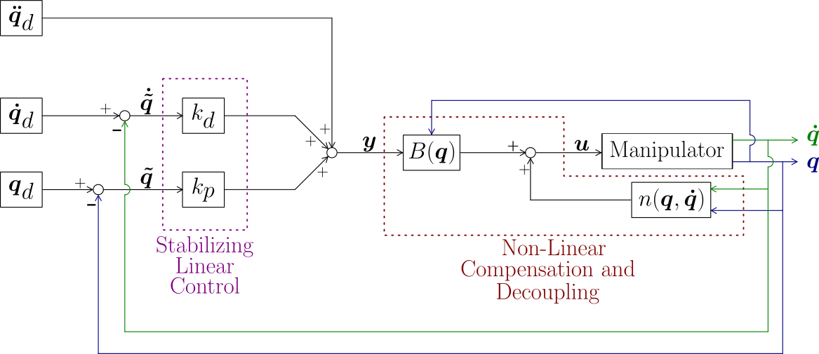
This control scheme allows to solve tracking problems.

Effectively, if we choose, \(\boldsymbol{r} = \ddot{\boldsymbol{q}}_d + K_D \dot{\boldsymbol{q}}_d + K_P \boldsymbol{q}_d\) then:

\[\ddot{\tilde{\boldsymbol{q}}} + K_D \dot{\tilde{\boldsymbol{q}}} + K_P \tilde{\boldsymbol{q}} = 0\]

which expresses the dynamics of the error \(\tilde{\boldsymbol{q}}\) while tracking the desired trajectory.

Note

1. \(B(\boldsymbol{q})\) and \(n(\boldsymbol{q}, \dot{\boldsymbol{q}})\) are computed online. This is computationally costly. Therefore, sometimes only the dominant terms are computed.

2. The approach is based on a perfect cancellation of the dynamics terms. This is difficult, or even not possible, if only the dominant terms are used. To overcome this problem, robust and adaptive methods are proposed:

• Robust control adds an additional term to counteract the effects of approximations.

• Adaptive control adapts the parameters of the model to the true values.