Feed-forward compensation
Based on Section 8.4 of Robotics: Modelling, Planning and Control.
The previous approach treats non-linearities and couplings as disturbances. These disturbances are known, however, and can be compensated.
Two approaches can be used, that are useful for tracking problems:
Decentralized feed-forward compensation
Computed torque feed-forward control
Decentralized feed-forward compensation
Position feedback control loop with decentralized feedforward compensation.
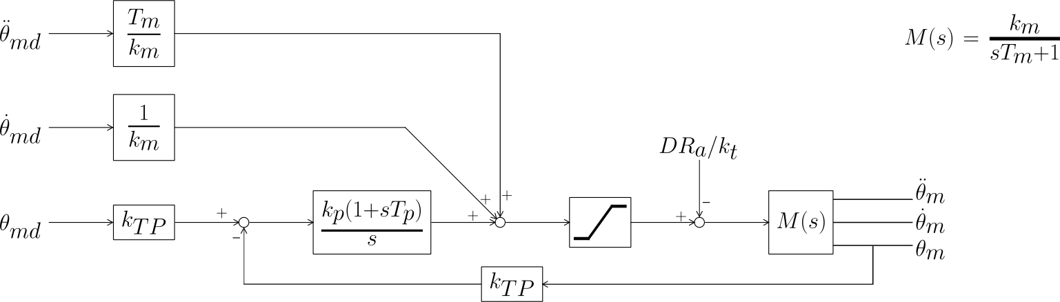
This schema greatly improves the performance of the tracking when high values of speed and acceleration are required.
We can check that the tracking is effectively achieved (\(\theta_m = \theta_{md}\)):
If position feedback is substituted by position/velocity/acceleration feedback, then the feedforward compensation requires less knowledge of the model (i.e., \(T_m\) and \(k_m\) values).
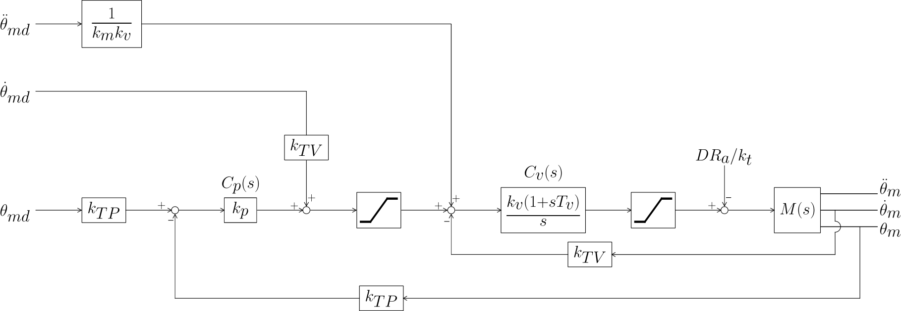
Computed torque feed-forward control
The idea is to add an extra term to the feedforward compensation that is able to compensate the disturbance itself, rather than its effects, by taking advantage of the dynamic model of the manipulator.
As detailed in the previous chapter, we had that:
with
where \(\boldsymbol{d}\) contains all the coupling terms, and that is a disturbance that can be anticipated by a feedforward term \(R_a k_t^{-1} \boldsymbol{d}_d\), with:
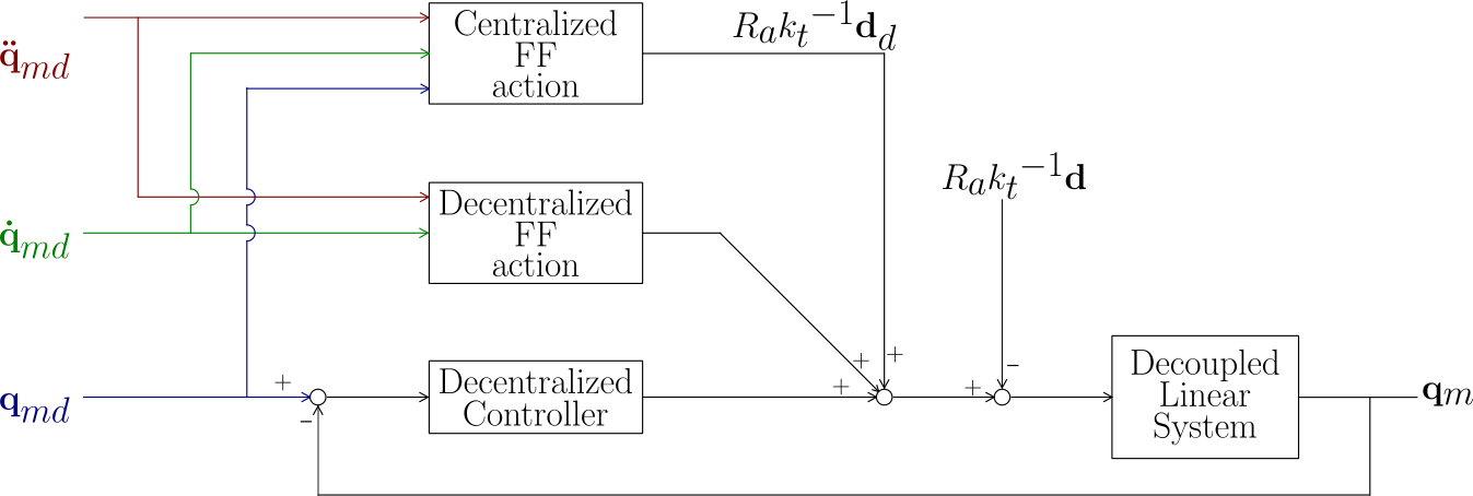
This centralized FF action:
Compensates the non-linear coupling due to the inertial, coriolis and centrifugal and gravitational terms that depend on the structure and that vary during the manipulator motion.
Is computationally costly: This cost can be reduced if only the gravitational part \(k_r^{-1} \boldsymbol{g}(\boldsymbol{q})\) and the diagonal terms of the inertial part \(k_r^{-1} \Delta B(\boldsymbol{q}) k_r^{-1}\) are computed.
Tends to compensate the disturbance (\(\boldsymbol{d}\)) and allows the control system to operate in a better condition. This is an inverse model strategy.