Force control

Based on Sections 9.1 and 9.2 of Robotics: Modelling, Planning and Control.

Needs and methods

The control of the interaction between the manipulator and the environment is crucial for the execution of tasks where:

  • The end-effector (EE) has to manipulate an object (e.g. assembly).

  • The EE has to perform an operation with a tool on a surface (e.g. polishing).

In these tasks, the environment sets constraints on the geometric paths that can be followed by the end-effector. Therefore, constrained motions have to be planned and controlled.

Using only a motion control strategy, the execution of the constrained motion tasks may fail because of unavailability of:

  • The accurate kinematic/dynamic model of the manipulator.

  • The accurate geometric model and mechanical features of the environment.

Force control is required, which can be:

  • Direct force control, like the hybrid force/motion strategies, when force measurements are available.

  • Indirect force control, like compliant control strategies, that rely on motion schemas.

Passive compliance

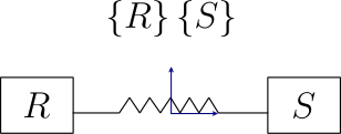
Consider two rigid bodies elastically coupled, with coincident reference frames in the absence of interaction forces and moments.
../../_images/4.5.1passive_compliance.svg

Consider now a relative displacement:

\[\begin{split}d \boldsymbol{x}_{rs} = \begin{bmatrix} d\boldsymbol{o}_{rs}\\ \boldsymbol{\omega}_{rs} \, dt \end{bmatrix} = d\boldsymbol{v}_{r,s} \, dt\end{split}\]

with \(d\boldsymbol{v}_{rs} = \boldsymbol{v}_s - \boldsymbol{v}_r\) being a vector of linear and angular velocities of S w.r.t. R.

The following force can be associated to this displacement:

\[\begin{split}\boldsymbol{h}_s = \begin{bmatrix} f_s \\ u_s \end{bmatrix} = \begin{bmatrix} k_f & k_c \\ k_c & k_{\mu} \end{bmatrix} \begin{bmatrix} d\,\boldsymbol{o}_{rs} \\ \boldsymbol{\omega}_{rs} \, dt \end{bmatrix} = K \boldsymbol{x}_{rs}\end{split}\]

where:

  • \(K\) = stiffness matrix

  • \(k_f\) = translational stiffness matrix

  • \(k_{\mu}\) = rotational stiffness matrix

  • \(k_c\) = coupling stiffness matrix

Also,

\[\boldsymbol{h}_r = -\boldsymbol{h}_s = - K d\boldsymbol{x}_{s,r}, \quad \text{with} \quad d \boldsymbol{x}_{r,s} = -d \boldsymbol{x}_{s,r}\]

Remote Center of Compliance (RCC)

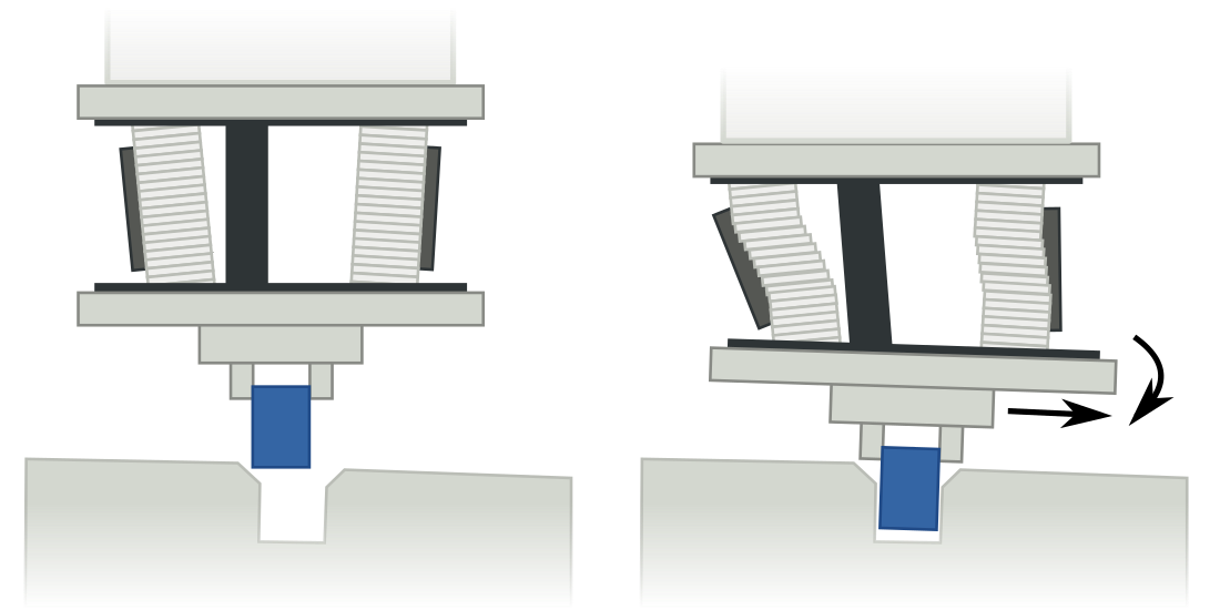
The Remote Center of Compliance (RCC) devices are devices mounted between the last link of the robot and the end-effector to introduce a passive compliance with the following features:

  1. Null coupling stiffness matrix

  2. High stiffness along some axis and low stiffness along the others, e.g., in a peg-in-a-hole task, we have a high stiffness along the axis of the hole and a low one along the others.

Te RCC devices convert contact forces into corrective motions.
../../_images/4.5.1RCC.png

Their disadvantage is their low versatility.

Active compliance

Use of a PD controller with gravity compensation scheme

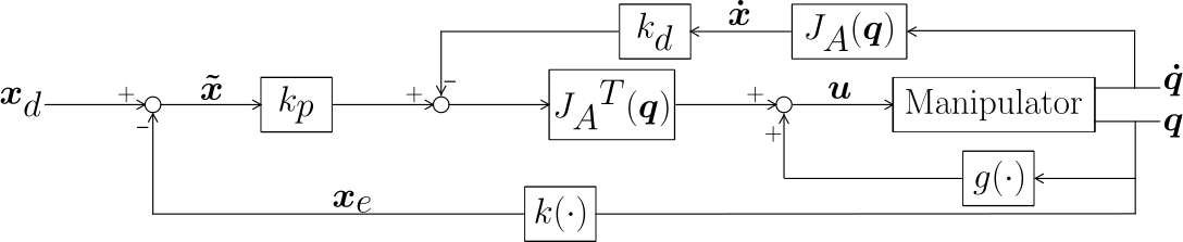
Consider the motion control scheme composed of a PD controller with gravity compensation in the operational space.
../../_images/4.5.2PD_opspace.svg

The control law is:

\[\boldsymbol{u} = \boldsymbol{g}(q) + J_A^T(\boldsymbol q) K_P \boldsymbol{\tilde x} - J_A^T(\boldsymbol q) K_D J_A(\boldsymbol q) \dot{\boldsymbol{q}}.\]

With \(K_P\) and \(K_D\) positive definite, the error tends asymptotically to zero.

If, however, a contact occurs, a reaction force appears between the end-effector and the environment, and the error cannot disappear.

Considering the reaction force \(\boldsymbol{h}_e\), the dynamic model of the manipulator is:

\[B(\boldsymbol q) \ddot{\boldsymbol{q}} + C(\boldsymbol q, \dot{\boldsymbol q}) \dot{\boldsymbol{q}} + F \dot{\boldsymbol{q}} + \boldsymbol{g}(\boldsymbol q) = \boldsymbol{u} + J^T(\boldsymbol q) \boldsymbol{h}_e\]

At the equilibrium (\(\dot{\boldsymbol{q}} = \boldsymbol{q} = 0\)), we have:

\[J^T(\boldsymbol q) \boldsymbol{h}_e = -J_A^T(\boldsymbol q) K_P \boldsymbol{x}\]

Recalling that:

\[J(\boldsymbol q) = T_A(\boldsymbol \phi_e) J_A(\boldsymbol q)\]

Then:

\[J_A^T(\boldsymbol q) \underbrace{T_A^T(\boldsymbol {\phi_e}) \boldsymbol{h}_e}_{\boldsymbol h_A} = -J_A^T(\boldsymbol q) K_P \boldsymbol{x}\]
\[\boxed{ \boldsymbol{h}_A = K_P \boldsymbol{\tilde x}}\]

That is, this control scheme behaves as a generalized spring in the operational space with stiffness \(K_P\).

Linear behavior in tranlation / non-linear behavior in orientation

If \(K_P\) is a diagonal matrix, then there is a linear behavior regarding translations, but not regarding rotations, since the equivalent forces \(\boldsymbol{h}_A\) depend on the end-effector orientation.

\[\begin{split}\boldsymbol{h}_A = T_A^T(\boldsymbol{\phi}_e) \boldsymbol{h}_e = \begin{bmatrix} I & 0 \\ 0 & T(\boldsymbol{\phi}_e) \end{bmatrix} \boldsymbol{h}_e\end{split}\]

With \(T(\boldsymbol{\phi}_e)\) dependant on the chosen Euler angles \((\varphi, \theta, \psi)\)), e.g.:

\[\begin{split}\text{For ZYZ: } T(\boldsymbol{\phi}_e) = \begin{pmatrix} 0 & -s_\varphi & c_\varphi s_\theta \\ 0 & c_\varphi & s_\varphi s_\theta \\ 1 & 0 & c_\theta \end{pmatrix}\end{split}\]
\[\begin{split}\text{For XYZ: } T(\boldsymbol{\phi}_e) = \begin{pmatrix} 1 & 0 & s_\theta \\ 0 & c_\varphi & -s_\varphi c_\theta \\ 0 & s_\varphi & c_\varphi c_\theta \end{pmatrix}\end{split}\]

Variant to achieve a linear behavior also in orientation

We can consider a new definition of the error in the operational space in order to achieve a linear behavior also in orientation and make it easy to define \(K_P\) for a given desired behavior:

Let \(T_e\) and \(T_d\) be the current and desired end-effector poses, respectively.

\[\begin{split}T_e = \begin{bmatrix} R_e & \boldsymbol{o}_e \\ \boldsymbol{0} & 1 \end{bmatrix} \qquad T_d = \begin{bmatrix} R_d & \boldsymbol{o}_d \\ \boldsymbol{0} & 1 \end{bmatrix}\end{split}\]

Then the current pose, \(T_e\), expressed w.r.t. the desired reference frame is:

\[\begin{split}T_d^e = T_d^{-1} T_e = \begin{bmatrix} R_e^d & {\boldsymbol{o}_{d,e}^d} \\ \boldsymbol{0} & 1 \end{bmatrix}\end{split}\]

with:

\[\boldsymbol{o}_{d,e} = R_d^T (\boldsymbol{o}_e - \boldsymbol{o}_d)\]
\[R_e^d = R_d^{-1} R_e\]

Now, let’s define the error \(\boldsymbol{\tilde{x}}\) (w.r.t. the desired reference frame):

\[\begin{split}\boldsymbol{\tilde{x}} = - \begin{bmatrix} \boldsymbol{o}^d_{d,e} \\ \boldsymbol{\phi}_{d,e} \end{bmatrix}\end{split}\]

where \(\boldsymbol{o}^d_{d,e}\) are the Euler angles corresponding to \(R^d_e\).

The time derivative \(\dot{\boldsymbol{\tilde{x}}}\) is computed as follows:

  1. Time derivative of \(\boldsymbol{o}^d_{d,e}\):

\[\dot{\boldsymbol{o}}^d_{d,e} = R_d^T (\boldsymbol{\dot o}_e - \boldsymbol{\dot o}_d) + \dot{R}_d^T (\boldsymbol{o}_e - \boldsymbol{o}_d) = R_d^T \dot{\boldsymbol{o}}_e \quad \text{(since the desired pose is considered constant)}\]
  1. Time derivative of \(\boldsymbol{\phi}_{d,e}\):

\[\dot{\boldsymbol{\phi}}_{d,e} = T^{-1}(\boldsymbol{o}_{d,e}) \boldsymbol{\omega}_{d,e} \quad \text{(recall that } T(\boldsymbol \phi) \text{ relates the angular velocities with the derivative of the Euler angles)}\]
\[\dot{\boldsymbol{\phi}}_{d,e} = T^{-1}(\boldsymbol{o}_{d,e}) R_d^T (\boldsymbol{\omega}_e - \boldsymbol{\omega}_d) \quad \text{(recall } R_d^T \dot{R}_d = 0 \text{ since the desired pose is constant)}\]
\[\boxed{ \dot{\boldsymbol{\phi}}_{d,e} = T^{-1}(\boldsymbol{\phi}_{d,e}) R_d^T \boldsymbol{\omega}_e}\]

In matrix form, \(\dot{\tilde{\boldsymbol{x}}}\) is:

\[\begin{split}\dot{\tilde{\boldsymbol{x}}} = - \begin{bmatrix} \dot{\boldsymbol{o}}^d_{d,e} \\ \boldsymbol{\phi}_{d,o} \end{bmatrix} = \begin{bmatrix} R_d^T & 0 \\ 0 & T^{-1}(\boldsymbol{\phi}_{d,e}) R_d^T \end{bmatrix} \begin{bmatrix} \boldsymbol{\dot o}_e \\ \boldsymbol{\omega}_e \end{bmatrix}\end{split}\]
\[\begin{split}= - \begin{bmatrix} I & 0 \\ 0 & T^{-1}(\boldsymbol{\phi}_{d,e}) \end{bmatrix} \begin{bmatrix} R_d^T & 0 \\ 0 & R_d^T \end{bmatrix} \boldsymbol{v}_e\end{split}\]
\[\begin{split}= - \underbrace{{T}_A^{-1}(\boldsymbol{\phi}_{d,c}) \begin{bmatrix} R_d^T & 0 \\ 0 & R_d^T \end{bmatrix} \begin{bmatrix} J(\boldsymbol{q}) \boldsymbol{\dot{q}} \end{bmatrix}}_{J_{Ad}(\boldsymbol{q}, \tilde{\boldsymbol{x}})}\end{split}\]
\[\boxed{ \dot{\tilde{\boldsymbol{x}}} = -{J}_{Ad}(\boldsymbol{q}, \dot{\tilde{\boldsymbol{x}}}) \boldsymbol{\dot{q}}}\]

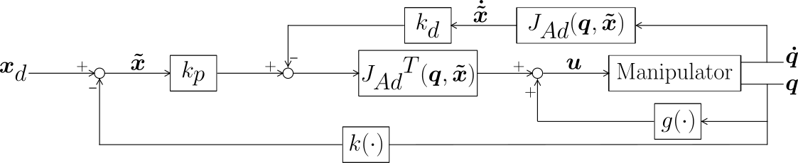
With this definition of the error, the control scheme and the control law are:
../../_images/4.5.3active_compliance.svg
\[\boldsymbol{u} = \boldsymbol{g}(\boldsymbol{q}) + {J}_{Ad}^T(\boldsymbol{q}, \dot{\tilde{\boldsymbol{x}}}) \left[ K_P \tilde{\boldsymbol{x}} - K_D {J}_{Ad}(\boldsymbol{q}, \tilde{\boldsymbol{x}}) \boldsymbol{\dot{q}} \right]\]

At the equilibrium point \((\boldsymbol{\dot q} = \boldsymbol{\ddot q} = 0)\) the dynamics is reduced to:

\[J^T(\boldsymbol{q}) \boldsymbol{h}_e = -J_{Ad}^T(\boldsymbol{q}, {\tilde{\boldsymbol{x}}}) K_P \tilde{\boldsymbol{x}}\]
\[\begin{split}J^T(\boldsymbol{q}) \boldsymbol{h}_e = - \left[ T_A^{-1}(\boldsymbol{\phi}_{de}) \begin{bmatrix} R_d^T & 0 \\ 0 & R_d^T \end{bmatrix} J(\boldsymbol{q}) \right]^T K_P \tilde{\boldsymbol{x}}\end{split}\]
\[\begin{split}J^T(\boldsymbol{q}) \boldsymbol{h}_e = -J^T(\boldsymbol{q}) \begin{bmatrix} R_d & 0 \\ 0 & R_d \end{bmatrix} T_A^{-T}(\boldsymbol{\phi}_{de}) K_P \tilde{\boldsymbol{x}}\end{split}\]
\[\begin{split}\underbrace{\begin{bmatrix} R_d^T & 0 \\ 0 & R_d^T \end{bmatrix} \boldsymbol{h}_e}_{\boldsymbol{h}_e^d} = -T_A^{-T}(\boldsymbol{\phi}_{de}) K_P \tilde{\boldsymbol{x}}\end{split}\]
\[\boxed{ \boldsymbol{h}_e^d = -T_A^{-T}(\boldsymbol{\phi}_{de}) K_P \tilde{\boldsymbol{x}}}\]

Now, consider a differential displacement \(d \tilde{\boldsymbol{x}} = \dot{\tilde{\boldsymbol{x}}} \big|_{\tilde{\boldsymbol{x}} = 0} dt\)

\[\begin{split}d \tilde{\boldsymbol{x}} = \dot{\tilde{\boldsymbol{x}}} \big|_{\tilde{\boldsymbol{x}} = 0} dt = -T_A^{-1}(\boldsymbol{0}) \underbrace{\begin{bmatrix} {R_d}^T & 0 \\ 0 & {R_d}^T \end{bmatrix} \boldsymbol{v}_e} dt\end{split}\]
\[= -T_A^{-1}(\boldsymbol{0}) \underbrace{\boldsymbol{v}_e^d} dt = -T_A^{-1}(\boldsymbol{0}) d {x}_{d,e}^d\]

If XYZ Euler angles are used then:

\[\begin{split}T_A(\boldsymbol{0}) = \begin{bmatrix} I_3 & 0_3 \\ 0_3 & T(\boldsymbol{0}) \end{bmatrix} =\left[ \begin{array}{c:ccc} I_3 & & 0_3 \\ \hdashline & 1 & 0 & s_{\boldsymbol{o}} \\ 0_3 & 0 & c_{\boldsymbol{\phi}} & -s_{\boldsymbol{\phi}} c_{\boldsymbol{o}} \\ & 0 & s_{\boldsymbol{\phi}} & c_{\boldsymbol{\phi}} c_{\boldsymbol{o}} \end{array} \right] = \begin{bmatrix} I_3 & 0_3 \\ 0_3 & I_3 \end{bmatrix} = I_6\end{split}\]

And:

\[\boldsymbol{h}_e^d = -T_A^{-T}(\boldsymbol{\phi}_{d,e}) K_P \tilde{\boldsymbol{x}} \quad (\tilde{\boldsymbol{x}}: \text{differential displacement})\]
\[= -\underbrace{T_A^{-T}(\boldsymbol{0})}_{I_6} K_P (-\underbrace{T_A^{-1}(\boldsymbol{0})}_{I_6} d {x}_{d,e}^d) = K_P d {x}_{d,e}^d\]

This is a decoupled active compliance scheme. \(K_P\) acts as a generalized spring between the current and desired EE poses, expressed in the desired reference frame.

Now a compliant behaviour can be easily defined from the geometry and mechanical features of the environment.

Compliant behaviour in a compliant environment

Consider now a compliant environment, i.e., the reaction force is proportional to the deformation of the environment:

\[\boldsymbol{h}_e = -K \, d {\boldsymbol{x}}_{e,r}\]

It can be illustrated with a two-link planar arm pushing a wall in the \(x\)-direction.
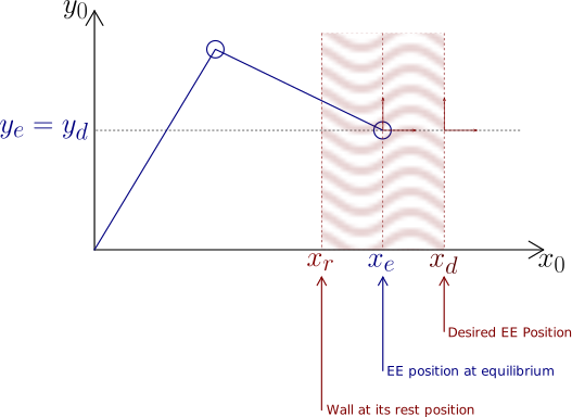
../../_images/4.5.4planararm_pushing_wall.svg

With a compliant control scheme, we have seen in the previous section that (dropping the supersindex):

\[d \boldsymbol{x}_{d,e} = K_P^{-1} \boldsymbol{h}_e\]
\[d \boldsymbol{x}_{d,e} = K_P^{-1} k \, d \boldsymbol{x}_{e,r}\]
\[d \boldsymbol{x}_{d,e} = K_P^{-1} k \left[ d \boldsymbol{x}_{d,r} - d \boldsymbol{x}_{d,e} \right]\]
\[\left( I + K_P^{-1} k \right) d \boldsymbol{x}_{d,e} = K_P^{-1} k \, d \boldsymbol{x}_{d,r}\]
\[d \boldsymbol{x}_{d,e} = \left( I + K_P^{-1} k \right)^{-1} K_P^{-1} k \, d \boldsymbol{x}_{d,r}\]
\[d \boldsymbol{x}_{d,e} = \left( K_P \left( I + K_P^{-1} k \right) \right)^{-1} k \, d \boldsymbol{x}_{d,r}\]
\[\boxed{d \boldsymbol{x}_{d,e} = (K_P + k)^{-1} k \, d \boldsymbol{x}_{d,r}}\]

The end-effector pose error \(d \boldsymbol{x}_{d,e}\) depends on the environment rest position \(\boldsymbol{x}_r\) and on the desired one \(\boldsymbol{x}_d\), and the interaction between the end-effector and the environment is influenced by the respective weight of the compliances coded in the (normally) diagonal matrices \(K_P\) and \(k\):

  1. In the direction of high stiffness of the manipulator (values of \(K_P\) greater than those of \(k\)), the environment complies and:

  • The manipulator is able to reach the desired pose:

\[d \boldsymbol{x}_{d,e} = (K_P + k)^{-1} k \, d \boldsymbol{x}_{d,r} \approx K_P^{-1} k \, d \boldsymbol{x}_{d,r} \rightarrow 0\]
  • The reaction force depends on the stiffness of the environment:

\[\boldsymbol{h}_e = K_P \, d \boldsymbol{x}_{d,e} = K_P (K_P + k)^{-1} k \, d \boldsymbol{x}_{d,r} \approx k \, d \boldsymbol{x}_{d,r}\]
  1. In the direction of low stiffness of the manipulator (values of \(K_P\) smaller than those of \(k\)), the manipulator complies and:

  • The manipulator is stopped at the environment rest position:

\[d \boldsymbol{x}_{d,e} = (K_P + k)^{-1} k \, d \boldsymbol{x}_{d,r} \approx d \boldsymbol{x}_{d,r}\]
  • The reaction force depends on the stiffness of the manipulator:

\[\boldsymbol{h}_e = K_P \, d \boldsymbol{x}_{d,e} = K_P (K_P + k)^{-1} k \, d \boldsymbol{x}_{d,r} \approx K_P \, d \boldsymbol{x}_{d,r}\]