TUTORIAL T3: Robot modelling, kinematics and differential kinematics
Based on chapter 2 and chapter 7 of Robotics, Vision and Control by Peter Corke.
Based on chapter 7 of Robotics, Vision and Control by Peter Corke.
Based on chapter 8 of Robotics, Vision and Control by Peter Corke.
It uses the The robotics toolbox for MATLAB.
Basic commands for representing position and orientation
Rotation matrices
>> R = rotx(pi/2)
>> trplot(R)
>> tranimate(R)
>> R = rotx(pi/2) * roty(pi/2)
>> trplot(R)
Euler angles ZYZ
Euler angles ZYZ ([\phi,\theta,\psi]) correspond to rotations about moved axes. The equivalent rotation matrix is R = R_z(\phi)R_{y'}(\theta)R_{z''}(\psi):
>> R = rotz(0.1)*roty(0.2)*rotz(0.3)
>> R = eul2r(0.1,0.2,0.3)
>> gamma = tr2eul(R)
>>> EXERCISE
Repeat with theta=-0.2. Note that a different set of Euler angles is returned, i.e. different sets of Euler angles give the same rotation matrix.
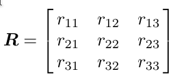
The expression of the rotation matrix as a function of the ZYZ-Euler angles is:

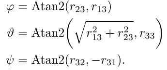
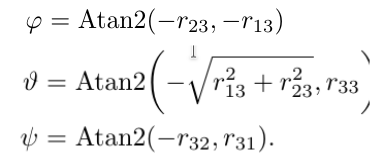
And the inverse problem is:
Euler angles RPY
Euler angles RPY ([\theta_r,\theta_p,\theta_y]) correspond to rotations about fixed axes: first \theta_y about x^W, then \theta_p about y^W, finally \theta_r about z^W,. The equivalent rotation matrix is R = R_z(\theta_r)R_y(\theta_p)R_x(\theta_y)
>> R = rotz(0.3)*roty(0.2)*rotx(0.1)
>> R = rpy2r(0.1,0.2,0.3,'zyx')
>> gamma = tr2rpy(R, 'zyx')
Since from version 10 of the Toolbox the ‘zyx’ is the default option, it could be omitted. If, instead, the parameter ‘xyz’ is passed to the rpy2r function then it considers a different definition of the RPY angles where the roll is about the x axis and the yaw about the y axis, i.e. R = R_x(\theta_r)R_y(\theta_p)R_z(\theta_y).
The expression of the rotation matrix as a function of the RPY-Euler angles is:

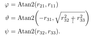
And the inverse problem is:

Axis-angle
>> R = angvec2r(pi/2,[1 0 0])
>> [theta,v] = tr2angvec(R)
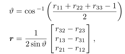
The expression of the rotation matrix as a function of the angle and axis is:

And the inverse problem is:
Quaternion
>> help UnitQuaternion
>> q1 = UnitQuaternion(R)
>> q1.R
>> q2 = q1.inv
>> q=q1*q2
>> q.R
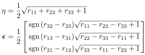
The expression of the rotation matrix as a function of the quaternion is:

And the inverse problem is:
Conversion functions
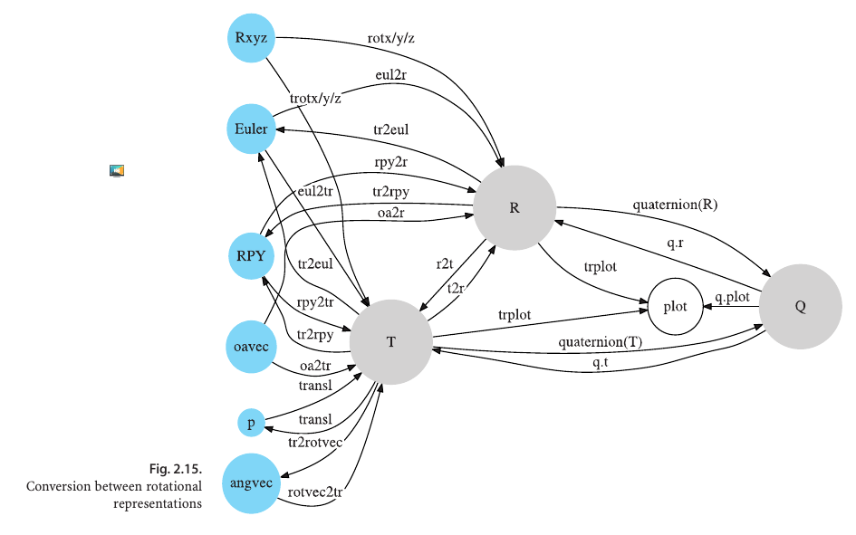
The following figure shows the conversion between all rotational representations offered by the Robotics Toolbox.
Homogeneous Transformations
The following functions create (4x4) matrices that represent homogeneous transformations:
>> T1 = transl(1, 0 ,0)
>> T2 = trotx(pi/2)
>> T = T1*T2
>> trplot(T)
>> R=t2r(T)
>> p=transl(T)
SE3
A class named SE3 is also provided to represent homogeneous transformations. It has many constructor methods, operators and also many operation, conversion, information methods:
>> TT1 = SE3(1,0,0)
>> TT2 = SE3.Rx(pi/2)
>> TTa = SE3(T)
>> about(T)
>> about(TTa)
>> TTb = TT1*TT2
>> res = TTa*TTb.inv
>> res.isidentity
>> help SE3
Robot modelling using DH parameters
The following video summarizes the reference frames used for the definition of the DH parameters used to model robotic manipulators:
The modelling of robotic manipulators is done as follows using the Robotics Toolbox:
Link parameters
- A link is defined with the function Link:
- L = Link(\theta,d,a,\alpha);
Two additional parameters can be added to specify the type of joint (0/1: revolute/prismatic, with default to 0) and the type of parameters (0/1: standard/modified, with default to 0). Other more explicit constructors are also provided (see the help for details):
>> help Link
>> L = Link([0, 0.1, 0.2, pi/2])
>> L = Link('revolute', 'd', 0.1, 'a', 0.2, 'alpha', pi/2);
>> L = Revolute('d', 1.2, 'a', 0.3, 'alpha', pi/2);
Evaluate the link frame for q=0.5:
>> L.A(0.5)
Add an offset to the joint angle and evaluate again:
>> L.offset = 0.5
>> L.A(0)
A two-link planar robot
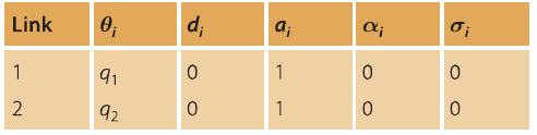
Consider a two-link planar arm with the following DH parameters:
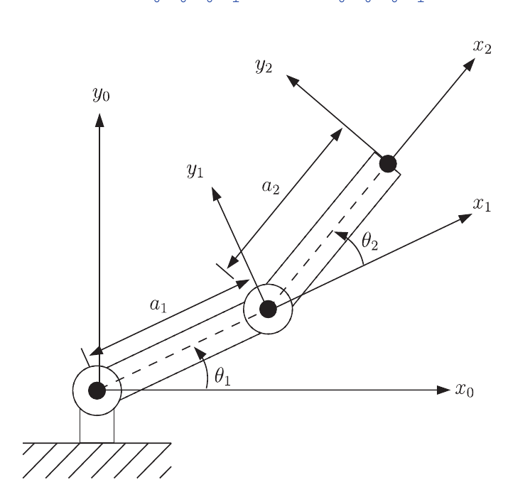
A function called SerialLink allows us to define kinematic structures:
>> L(1) = Link([0 0 1 0]);
>> L(2) = Link([0 0 1 0]);
>> L
>> twolink = SerialLink(L, 'name', 'two link')
Another manipulator can be create from an existing one:
>> clone = SerialLink(twolink,'name','twin')
The manipulator can be ploted and interactively moved:
>> help SerialLink
>> twolink.plot([0,0])
>> twolink.teach
Some few robot models are already available in the Toolbox, that can be instantiated just by running a script, thus avoiding the need to create them:
>> clear
>> mdl_twolink
>> twolink.n
>> L = twolink.links
>> twolink.display
Procedure to determine the DH parameters

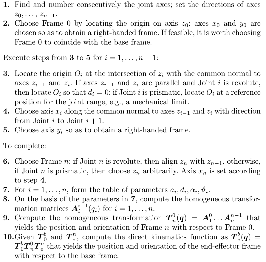
DH parameters convention:
DH parameters for an anthropomorphic arm:
Forward kinematics
The two link planar robot
Use the script provided by the toolbox to load the two-link planar robot:
>> mdl_twolink
>> twolink
Compute the forward kinematics and plot:
>> twolink.fkine([0,0])
>> twolink.plot([0,0])
>> twolink.fkine([pi/4,pi/4])
>> twolink.plot([pi/4,pi/4])
The PUMA 560 robot
Use the script provided by the toolbox to load the PUMA 560 robot and the frequently used configurations qz, qr, qs and qn:
>> mdl_puma560
>> p560
>> p560.plot(qz)
>> p560.plot(qr)
>> p560.plot(qs)
>> p560.plot(qn)
Compute the forward kinematics at qz using the fkine method that returns an SE3 element. Clone the robot and repeat after defining a Tool and a Base for the new robot. Verify the differences in the homogeneous transforms.
>> T1 = p560.fkine(qz)
>> p560b = SerialLink(p560, 'name', 'Puma 560b');
>> p560b.tool = transl(0,0,0.2)
>> T2 = p560b.fkine(qz)
>> p560b.base = transl(0,0,1)
>> T3 = p560b.fkine(qz)
>> p560.plot(qz)
>> figure
>> p560b.plot(qz, 'workspace', [-1,1,-1,1,-1,2])
Inverse kinematics
Closed form using the Toolbox
The ikine6s function of the SerialLink class gives a closed form solution of the inverse kinematics for six DOF manipulators with spherical wrist like the Puma 560:
>> qn
>> T = p560.fkine(qn)
>> q1 = p560.ikine6s(T)
Note that q1 is different from qn.
The eight different inverse kinematic solutions can be obtained by specifying:
- r/l: right arm / left arm.
- u/d: elbow up / elbow down.
- f/n: flipped wrist / not flipped wrist.
The default values are: l, u and n.
>> q2 = p560.ikine6s(T, 'ru')
>>> EXERCISE
    Check the other solutions solutions and plot them.
Numerical solution
The ikine function of the SerialLink class gives a numerical solution using differential kinematics, and therefore is useful for any kind of manipulators.
>> qn
>> T = p560.fkine(qn)
>> q1 = p560.ikine(T)
Note that the solution q1 is different from qn. In this case the solution found has the elbow down. With this numerical solution, the solution found depends on the initial configuration (which is defaulted to zero), and can not be explicitly controlled although different solutions can be found by changing the initial configuration:
>> q2 = p560.ikine(T, 'q0', [0 0 3 0 0 0])
>>> EXERCISE
    Check the forward and inverse kinematics for the Universal Robot's UR3.
Geometric Jacobian
The anthropomorphic arm


The Jacobian for three revolute joints is:
J(\mathbf{q}) = \left[ {\begin{array}{c} J_p(\mathbf{q}) \\ J_{\Theta}(\mathbf{q}) \\ \end{array} } \right] = \left[ {\begin{array}{ccc} \mathbf{z}_0 \times (\mathbf{p}_e - \mathbf{p}_0) & \mathbf{z}_1 \times (\mathbf{p}_e - \mathbf{p}_1) & \mathbf{z}_2 \times (\mathbf{p}_e - \mathbf{p}_2) \\ \mathbf{z}_0 & \mathbf{z}_1 & \mathbf{z}_2 \\ \end{array} } \right]
The homogeneous transformations between links are:
A_1^{0}(q_1) = \left[ {\begin{array}{cccc} c_1 & 0 & s_1 & 0 \\ s_1 & 0 & -c_1 & 0 \\ 0 & 1 & 0 & 0 \\ 0 & 0 & 0 & 1 \\ \end{array} } \right],\;\;\;\;\; A_i^{i-1}(q_i) = \left[ {\begin{array}{cccc} c_i & -s_i & 0 & a_i c_i \\ s_i & c_i & 0 & a_i s_i \\ 0 & 0 & 1 & 0 \\ 0 & 0 & 0 & 1 \\ \end{array} } \right] \;\;\; i=2,3.
The origin \mathbf{\tilde{p}}^i_i=[0\; 0\; 0\; 1]^T of the reference frame of link i\in \{0..3\} is represented in the base frame as:
\mathbf{\tilde{p}}_0 = \left[ {\begin{array}{c} 0 \\ 0 \\ 0 \\ 1 \\ \end{array} } \right],\;\;\; \mathbf{\tilde{p}}_1 = A_1^{0}(q_1)\mathbf{\tilde{p}}^1_1 = \left[ {\begin{array}{c} 0 \\ 0 \\ 0 \\ 1 \\ \end{array} } \right],\;\;\; \mathbf{\tilde{p}}_2 = A_1^{0}(q_1)A_2^{1}(q_2)\mathbf{\tilde{p}}^2_2 = \left[ {\begin{array}{c} a_2 c_1 c_2 \\ a_2 s_1 c_2 \\ a_2 s_2 \\ 1 \\ \end{array} } \right],\;\;\; \mathbf{\tilde{p}}_e =\mathbf{\tilde{p}}_3 = A_1^{0}(q_1)A_2^{1}(q_2)A_3^{2}(q_3)\mathbf{\tilde{p}}^3_3 = \left[ {\begin{array}{c} c_1 (a_2 c_2 + a_3 c_{23}) \\ s_1 (a_2 c_2 + a_3 c_{23}) \\ a_2 s_2 + a_3 s_{23} \\ 1 \\ \end{array} } \right].
The z-axes of the link reference frames are:
\mathbf{z}_0 = \left[ {\begin{array}{c} 0 \\ 0 \\ 1 \\ \end{array} } \right],\;\;\; \mathbf{z}_1 = R_1^{0}(q_1)\mathbf{z}_0 = \left[ {\begin{array}{c} s_1 \\ -c_1 \\ 0 \\ \end{array} } \right],\;\;\; \mathbf{z}_2 = R_1^{0}(q_1)R_2^{0}(q_2)\mathbf{z}_0 = \left[ {\begin{array}{c} s_1 \\ -c_1 \\ 0 \\ \end{array} } \right].
Then, the Jacobian results:
J(\mathbf{q}) = \left[ {\begin{array}{ccc} -s_1 (a_2 c_2 + a_3 c_{23}) & -c_1 (a_2 s_2 + a_3 s_{23}) & -a_3 c_1 s_{23}\\ c_1 (a_2 c_2 + a_3 c_{23}) & -s_1 (a_2 s_2 + a_3 s_{23}) & -a_3 s_1 s_{23} \\ 0 & a_2 c_2 + a_3 c_{23} & a_3 c_{23}\\ 0 & s_1 & s_1 \\ 0 & -c_1 & -c_1 \\ 1 & 0 & 0 \\ \end{array} } \right]
Using the robotics toolbox
The Robotics Toolbox provides a method in the SerialLink class that allows to compute the Geometric Jacobian at a given configuration:
>> mdl_puma560
>> J = p560.jacob0(qn)
The Geometric Jacobian J(\mathbf{q}) relates the joint velocities \dot{\mathbf{q}} with the end-effector linear and angular velocities \mathbf{v}=(\dot{x},\dot{y},\dot{z},\omega_x,\omega_y,\omega_z)^T. The function jacbo0 gives the Cartesian velocities of the end-effector measured from the base frame (hence the 0 in the name of the function)
The rows of J are the Cartesian degrees of freedom and the columns the joints, therefore for the 6 degree of freedom Puma 560 manipulator the Jacobian is a (6x6) square matrix.
The (3x3) zero block indicates that the joint velocities of the wrist joints do not have any effect on the linear motion of the end-effector.
The joint velocities required to move along a small velocity in the z-direction are:
>> qd = inv(J)*[0 0 0.1 0 0 0]'
As an example, the robot can be moved along a given velocity v_base defined w.r.t. the base using the Jacobian as follows:
>> v_base = [1,0,0,0,0,0]'
>> Delta = 0.007;
>> qcurrent=qn;
>> qpath=[qcurrent];
>> for i=1:20
>>  qdot=inv(p560.jacob0(qcurrent))*v_base;
>>  qnext = qcurrent + Delta*qdot';
>>  qpath=[qpath; qnext];
>>  qcurrent = qnext;
>> end
>> p560.plot(qpath)
>>> EXERCISE
  Write a Matlab function called qdot that has as input a serial link, a configuration and a desired operational space velocity and returns the joint velocities.
Analytic Jacobian
The anthropomorphic arm
The Analytical Jacobian is:
J_A(\mathbf{q}) = \left[ {\begin{array}{c} J_p(\mathbf{q}) \\ J_{\Phi}(\mathbf{q}) \\ \end{array} } \right] = \left[ {\begin{array}{c} \frac{\partial \mathbf{p}_e}{\partial \mathbf{q}} \\ \frac{\partial \mathbf{\Phi}_e}{\partial \mathbf{q}} \\ \end{array} } \right]
The position of the end effector is:
\mathbf{p}_e = \left[ {\begin{array}{c} c_1 (a_2 c_2 + a_3 c_{23}) \\ s_1 (a_2 c_2 + a_3 c_{23}) \\ a_2 s_2 + a_3 s_{23} \end{array} } \right]
Then, the linear part of the analytical Jacobian becomes:
J_p(\mathbf{q}) = \left[ {\begin{array}{ccc} \frac{\partial x}{\partial q_1} & \frac{\partial x}{\partial q_2} & \frac{\partial x}{\partial q_3} \\ \frac{\partial y}{\partial q_1} & \frac{\partial y}{\partial q_2} & \frac{\partial y}{\partial q_3} \\ \frac{\partial z}{\partial q_1} & \frac{\partial z}{\partial q_2} & \frac{\partial z}{\partial q_3} \\ \end{array} } \right] = \left[ {\begin{array}{ccc} -s_1 (a_2 c_2 + a_3 c_{23}) & -c_1 (a_2 s_2 + a_3 s_{23}) & -c_1 a_3 s_{23}\\ c_1 (a_2 c_2 + a_3 c_{23}) & -s_1 (a_2 s_2 + a_3 s_{23}) & -s_1 a_3 s_{23}\\ 0 & a_2 c_2 + a_3 c_{23} & a_3 c_{23} \end{array} } \right]
The orientation of the end effector is:
\mathbf{\Phi}_e = \left[ \begin{array}{ccc} c_1 c_{23} & -c_1 s_{23} & s_1 \\ s_1 c_{23} & -s_1 s_{23} & -c_1 \\ s_{23} & c_{23} & 0 \end{array} \right] = \left[ \begin{array}{ccc} r_{11} & r_{12} & r_{13} \\ r_{21} & r_{22} & r_{23} \\ r_{31} & r_{32} & r_{33} \\ \end{array} \right]
The corresponding ZYZ Euler angles are:
\begin{array}{rcl} \phi & = & \textrm{atan2}(r_{23},r_{13}) = \textrm{atan2}(-c_1,s_1) = q_1 - \frac{\pi}{2}\\ \theta & = & \textrm{atan2}(\sqrt{r_{13}^2 + r_{23}^2}, r_{33}) = \textrm{atan2}(1,0) = \frac{\pi}{2}\\ \psi & = & \textrm{atan2}(r_{32},-r_{31}) = \textrm{atan2}(c_{23},-s_{23}) = q_2+q_3+\frac{\pi}{2}\\ \end{array}
Then, the angular part of the analytical Jacobian becomes:
J_\Phi(\mathbf{q}) = \left[ {\begin{array}{ccc} \frac{\partial \phi}{\partial q_1} & \frac{\partial \phi}{\partial q_2} & \frac{\partial \phi}{\partial q_3} \\ \frac{\partial \theta}{\partial q_1} & \frac{\partial \theta}{\partial q_2} & \frac{\partial \theta}{\partial q_3} \\ \frac{\partial \psi}{\partial q_1} & \frac{\partial \psi}{\partial q_2} & \frac{\partial \psi}{\partial q_3} \\ \end{array} } \right] = \left[ {\begin{array}{ccc} 1 & 0 & 0\\ 0 & 0 & 0\\ 0 & 1 & 1\\ \end{array} } \right]
It can be verified that it corresponds to the angular part of the Geometric Jacobian computed above, which are related through matrix T_A(\Phi).
J_\Theta(\mathbf{q}) = T(\Phi) J_\Phi(\mathbf{q}) = \left[ {\begin{array}{ccc} 0 & -s_\phi & c_\phi s_\theta \\ 0 & c_\phi & s_\phi s_\theta \\ 1 & 0 & c_\theta \\ \end{array} } \right] \left[ {\begin{array}{ccc} 1 & 0 & 0\\ 0 & 0 & 0\\ 0 & 1 & 1\\ \end{array} } \right] = \left[ {\begin{array}{ccc} 0 & c_\phi s_\theta & c_\phi s_\theta \\ 0 & -s_\phi s_\theta & -s_\phi s_\theta \\ 1 & c_\theta & c_\theta \\ \end{array} } \right]
Since \phi=q_1-\frac{\pi}{2} and \theta=\frac{\pi}{2}, then c_\phi=s_1, s_\phi=-c_1, c_\theta=0, and s_\theta=1. Therefore, as expected:
J_\Theta(\mathbf{q}) = \left[ {\begin{array}{ccc} 0 & s_1 & s_1 \\ 0 & -c_1 & -c_1 \\ 1 & 0 & 0 \\ \end{array} } \right]
Using the robotics toolbox
The jacob0 method introduced before, gives us the Analytical Jacobian if the parameter `eul` is added:
>> JA = p560.jacob0(qn,'eul')
The relation between the Geometric Jacobian and the Analytic Jacobian is:
J = T_A(\Phi_e) J_A = \left[ {\begin{array}{cc} \mathbf{I}_3 & \mathbf{0}_3 \\ \mathbf{0}_3 & T(\Phi_e) \\ \end{array} } \right] J_A
The Toolbox provides the function eul2jac(phi,theta,psi) that implements the matrix T(\Phi_e), with \Phi_e being the ZYZ Euler angles \Phi_e = [\phi,\theta,\psi]^T.
>> Tn = p560.fkine(qn)
>> Phi_e = Tn.toeul
>> TA = J*inv(JA)
>> T = TA(4:6,4:6)
>> T = eul2jac(Phi_e)
Alternatively to the use of ZYZ Euler angles, RPY angles can be used, and then the expression of the analytical Jacobian and that of matrix T(\Phi_e) vary. Matrix T(\Phi_e) is implemented in the robotics toolbox by the function rpy2jac.
Transforming Velocities between Coordinate Frames
The Jacobian
Consider two frames {A} and {B} related by:
^A T_B = \left[ {\begin{array}{cc} \mathbf{R} & \mathbf{t} \\ 0 & 1 \\ \end{array} } \right]
Then a spatial velocity (or twist) with respect to frame {A} can be expressed relative to frame {B} by:
^B v = \; ^B J_A(\;^A T_B) \;\; ^A v = \left[ {\begin{array}{cc} \mathbf{R}^T & (\mathbf{S}(\mathbf{t})\mathbf{R})^T \\ \mathbf{0}_3 & \mathbf{R}^T \\ \end{array} } \right] \;\; ^A v
where
\mathbf{S}(\mathbf{t}) = \left[ {\begin{array}{ccc} 0 & -t_z & t_y \\ t_z & 0 & -t_x \\ -t_y & t_x & 0 \\ \end{array} } \right]
See pages 174 and 175 of Robotics, Vision and Control by Peter Corke, and pages 149-151 of Robotics: Modelling, planning and control by B. Siciliano et al.
Spacial velocities (or twists) can be composed if they are expressed in the same reference frame. Therefore, this is a useful tool to convert all of them to the same reference frame.
Using the robotics toolbox
The robotics toolbox includes the function tr2jac that computes the above Jacobian. It has as parameter the transform between frame {A} and {B}:
>> T_AB = transl(1, 0, 0)*troty(pi/2);
>> J_BA = tr2jac(T_AB)
>> vA = [1 0 0 0 0 0]';
>> vB = J_BA*vA;
>>> EXERCISE
      Check that effectively  tr2jac implements the matrix shown above.
As an example consider the Base frame of the robot as frame {B} and the Tool frame as frame {A}. A velocity defined in the Tool reference frame can then be expressed in the Base frame:
>> clear;
>> mdl_puma560;
>> q=[0,pi/2,-pi/4,0,pi/4,0]
>> p560.plot(q)
>> v_tool=[0,0,1,0,0,0]'
>> T=p560.fkine(q)
>> Jv=tr2jac(inv(T))
>> v_base=Jv*v_tool
Then, using the Jacobian of the robot, it can be moved along the velocity v_base:
>> Delta = 0.007;
>> qcurrent=q;
>> qpath=[q];
>> for i=1:10
>>  qdot=inv(p560.jacob0(qcurrent))*v_base;
>>  qnext = qcurrent + Delta*qdot';
>>  qpath=[qpath; qnext];
>>  qcurrent = qnext;
>> end
>> p560.plot(qpath)
>>> EXERCISE
    1) Test for other velocities.
    2) Try to move the robot along a velocity composed of a velocity along the z-axis of the tool and another along the z-axis of the base.