Basic issues
Linear algebra
Matrices
- If \mathbf{A} and \mathbf{B} are two matrices, then:
\begin{aligned} (\mathbf{A}\mathbf{B})^T &= \mathbf{B}^T\mathbf{A}^T \\ (\mathbf{A}\mathbf{B})^{-1} &= \mathbf{B}^{-1}\mathbf{A}^{-1} \\ \mathbf{A}^{-T} &= (\mathbf{A}^{-1})^T = (\mathbf{A}^T)^{-1} \end{aligned}
- A skew-symmetric (or antisymmetric) matrix is a square matrix \mathbf{A} whose transpose is also its negative; that is, it satisfies the condition -\mathbf{A} = \mathbf{A}^T.
If \mathbf{p}=(x,y,z)^T, then the skew-symmetric operator \mathbf{S} is defined as:
\mathbf{S}(\mathbf{p}) = \left( \begin{array}{rrr} 0 & -z & y \\ z & 0 & -x \\ -y & x & 0 \\ \end{array} \right)
The following is satisfied: \mathbf{q}^T \mathbf{S}(\mathbf{p})\mathbf{q}=0.
- A positive definite matrix \mathbf{A} is a n\times n square symmetric matrix that satisfies \mathbf{z}^T \mathbf{A} \mathbf{z} >0 for any n\times 1 vector \mathbf{z}.
Gradient
Let f(\mathbf{x}) be a scalar function of \mathbf{x}=(x_1,\dots,x_n)^T. Then, the gradient of function f w.r.t. \mathbf{x} is:
\nabla_x f(\mathbf{x})=\left( \frac{\partial f(\mathbf{x})}{\partial \mathbf{x}}\right)^T =\left( \frac{\partial f(\mathbf{x})}{\partial x_1}, \dots, \frac{\partial f(\mathbf{x})}{\partial x_n}\right)^T
and:
\dot{f}(\mathbf{x}) = \frac{d}{dt}f(\mathbf{x})=\nabla_x f(\mathbf{x}) \dot{\mathbf{x}}
Jacobian
Let \mathbf{g}(\mathbf{x}) be a vector of m functions g_1(\mathbf{x}),\dots,g_m(\mathbf{x}) of \mathbf{x}=(x_1,\dots,x_n)^T. Then, the Jacobian is the m\times n matrix:
\mathbf{J} = \frac{\partial \mathbf{g}(\mathbf{x})}{\partial \mathbf{x}}=\left( \begin{array}{c} \frac{\partial g_1(\mathbf{x})}{\partial \mathbf{x}} \\ \vdots \\ \frac{\partial g_m(\mathbf{x})}{\partial \mathbf{x}} \\ \end{array} \right) = \left( \begin{array}{ccc} \frac{\partial f_1(\mathbf{x})}{\partial x_1} & \dots & \frac{\partial f_m(\mathbf{x})}{\partial x_n} \\ \vdots & & \vdots \\ \frac{\partial f_1(\mathbf{x})}{\partial x_1} & \dots &\frac{\partial f_m(\mathbf{x})}{\partial x_n} \\ \end{array} \right)
Linear transformations
Let \mathbf{y}=\mathbf{A}\mathbf{x},\;\; \mathbf{x}\in \mathcal{X},\;\;\mathbf{y}\in \mathcal{Y} with \mathcal{X} and \mathcal{Y} vector spaces of dimension n and m respectively, and \mathbf{A} a m\times n matrix.
The range space of \mathbf{A} is:
\mathcal{R}(\mathbf{A}) = \{ \mathbf{y}:\mathbf{y}=\mathbf{A}\mathbf{x}, \mathbf{x}\in \mathcal{X}\}\subseteq \mathcal{Y}.
The rank of \mathbf{A} is the dimension of the range space:
\rho(\mathbf{A}) = \textrm{dim}\{\mathcal{R}(\mathbf{A})\}.
The null space of \mathbf{A} is:
\mathcal{N}(\mathbf{A}) = \{ \mathbf{x}: \mathbf{A}\mathbf{x}=0, \mathbf{x}\in \mathcal{X}\}\subseteq \mathcal{X}.
The follow holds:
\textrm{dim}\{\mathcal{R}(\mathbf{A})\} + \textrm{dim}\{\mathcal{N}(\mathbf{A})\} = n.
Eigenvalues and eigenvectors
Let \mathbf{A} be a n\times n matrix, and \textrm{det}(\lambda \mathbf{I}-\mathbf{A})=0 its characteristic equation.
The eigenvalues of \mathbf{A} are the solutions (\lambda_1,\dots,\lambda_n) of the characteristic equation.
The eigenvectors of \mathbf{A} are the solution of (\lambda_i \mathbf{I}-\mathbf{A})\mathbf{u}_i=0,i=1,\dots,n.
If \mathbf{U}=[\mathbf{u}_1,\dots,\mathbf{u}_n], then:
\Lambda =\mathbf{ U}^{-1}\mathbf{A} \mathbf{U}=\textrm{diag}\{\lambda_1,\dots,\lambda_n\}.
Pseudo-inverses
Let \mathbf{A} be a m\times n matrix. Then:
- If m<n, the right-inverse of \mathbf{A} is the matrix \mathbf{A}^\dag_r satisfying:
\mathbf{A}\mathbf{ A}^\dag_r = \mathbf{I}_m.
- If m>n, the left-inverse of \mathbf{A} is the matrix \mathbf{A}^\dag_l satisfying:
\mathbf{A}^\dag_l \mathbf{A} = \mathbf{I}_n.
Their expressions are:
\begin{aligned} \mathbf{A}^\dag_r &=& \mathbf{A}^T (\mathbf{A} \mathbf{A}^T)^{-1} \nonumber \\ \mathbf{A}^\dag_l &=& (\mathbf{A}^T \mathbf{A})^{-1} \mathbf{A}^T \nonumber \end{aligned}
And the corresponding weighted expressions are:
\begin{aligned} \mathbf{A}^\dag_r &=& \mathbf{W}_r^{-1} \mathbf{A}^T (\mathbf{A} \mathbf{W}_r^{-1} \mathbf{A}^T)^{-1} \nonumber\\ \mathbf{A}^\dag_l &=& (\mathbf{A}^T \mathbf{W}_l \mathbf{A})^{-1} \mathbf{A}^T \mathbf{W}_l \nonumber \end{aligned}
with \mathbf{W}_r and \mathbf{W}_l positive definite matrices of dimension n and m, respectively.
Single-value decompositions (SVD)
Let \mathbf{A} be a m\times n matrix. Then, \mathbf{A}^T\mathbf{A} has n non-negative eigenvalues \lambda_1\geq\lambda_s\dots\lambda_n\geq 0.
Let \lambda_i = \sigma_i^2, \; \sigma_i\geq 0. The \sigma_i are called the singular values of \mathbf{A}.
The SVD of a matrix \mathbf{A} is:
\begin{array}{ccl} \mathbf{A} &=& \mathbf{U} \Sigma \mathbf{V}^T \\ \mathbf{U} &=& [\mathbf{u}_1,\dots,\mathbf{u}_m] = \textrm{ eigenvectors of } \mathbf{A}\mathbf{A}^T\\ \mathbf{V} &=& [\mathbf{v}_1,\dots,\mathbf{v}_n] = \textrm{ eigenvectors of } \mathbf{A}^T\mathbf{A}\\ \mathbf{\Sigma} &=& \left( \begin{array}{cc} \mathbf{D} & 0 \\ 0 & 0 \\ \end{array} \right) = n\times n \textrm{ matrix}\\ \mathbf{D} &=& \textrm{diag}\{\sigma_1,\dots,\sigma_{rank(\mathbf{A})}\} \end{array}
SVD constructs orthonormal basis of the range and the null spaces of \mathbf{A}:
- The columns of \mathbf{U} corresponding to non-zeros singular values form an othonormal basis of \mathcal{R}(\mathbf{A}).
- The columns of \mathbf{V} corresponding to null singular values form an othonormal basis of \mathcal{N}(\mathbf{A}).
Then, the solution of \mathbf{A}\mathbf{h}=0 satisfies \mathbf{h}\in \mathcal{N}(\mathbf{A}) and therefore is a linear combination of the columns of \mathbf{V} corresponding to the null singular values of \mathbf{A}.
Operational space vs. joint space
Concepts
The configuration of a robot in the joint space is (q_1,\dots,q_n)^T.
The configuration of the robot in the operational space is determined by the pose (position and orientation) of the end-effector (EE) w.r.t. a fixed reference frame. If the robot workspace is \bm{R}^3 then the pose can be expressed as a 6\times 1 vector:
\mathbf{x}_e = \left( \begin{aligned} \mathbf{p}_e \\ \bm{\phi}_e \\ \end{aligned} \right)
where \mathbf{p}_e=(x,y,z)^T determines the position, and \bm{\phi}_e=(\varphi,\upsilon,\psi)^T a minimal representation of the orientation (e.g. using ZYZ Euler angles).
Representation of orientations
Rotation matrix
A 3\times 3 matrix composed of the three unit vectors describing the rotated reference frame w.r.t the fixed reference frame:
\mathbf{R}=(x', y', z')
The following holds:
\begin{aligned} \mathbf{R}^{-1}=\mathbf{R}^T\\ \textrm{det}(\mathbf{R})=1. \end{aligned}
Rotation around the z, y and x-axis are:
\mathbf{R}_z(\alpha) = \left( \begin{array}{ccc} c\alpha & -s\alpha & 0 \\ s\alpha & c\alpha & 0 \\ 0 & 0 & 1 \\ \end{array} \right)
\mathbf{R}_y(\beta) = \left( \begin{array}{ccc} c\beta & 0 & -s\beta \\ 0 & 1 & 0 \\ s\beta & 0 & c\beta \\ \end{array} \right)
\mathbf{R}_x(\gamma) = \left( \begin{array}{ccc} 1 & 0 & 0 \\ 0 & c\gamma & -s\gamma \\ 0 & s\gamma & c\gamma \\ \end{array} \right)
The time-derivative of \mathbf{R} is \dot{\mathbf{R}}=\mathbf{S}(w)\mathbf{R}, \mathbf{S}(\omega) being the skew-symmetric operator:
\mathbf{S}(\bm{\omega})= \left( \begin{array}{ccc} 0 & -\omega_z & \omega_y \\ \omega_z & 0 & -\omega_x \\ -\omega_y & \omega_x & 0 \\ \end{array} \right)
Euler angles \bm{\phi}=(\varphi,\upsilon,\psi)
Consecutive rotations around the axis of the rotated frame.
The rotation matrix is obtained by post-multiplications.
For the ZYZ case:
\mathbf{R}(\bm{\phi}) = \mathbf{R}_z(\varphi)\mathbf{R}_{y'}(\upsilon)\mathbf{R}_{z''}(\psi).
For the XYZ case:
\mathbf{R}(\bm{\phi}) = \mathbf{R}_x(\varphi)\mathbf{R}_{y'}(\upsilon)\mathbf{R}_{z''}(\psi).
Roll-pitch-yaw:
Consecutive rotations around the x, y and z axis of the fixed frame.
The rotation matrix is obtained by pre-multiplications:
\mathbf{R}(\bm{\phi}) = \mathbf{R}_z(\varphi)\mathbf{R}_{y}(\upsilon)\mathbf{R}_{x}(\psi).
Homogeneous transformations
Let \mathbf{\tilde{p}} be the homogeneous representation of a vector \mathbf{p}:
\mathbf{\tilde{p}}=\left( \begin{array}{c} \mathbf{p} \\ 1 \\ \end{array} \right)
Then, the homogeneous transformation \mathbf{A}^0_1 defines the position and orientation of a frame \{1\} with respect to another frame \{0\}:
\mathbf{A}^0_1 = \left( \begin{array}{cc} \mathbf{R}^0_1 & \mathbf{o}^0_1 \\ \mathbf{0}^T & 1 \\ \end{array} \right)
Geometric Jacobian
The geometric jacobian \mathbf{J}(\mathbf{q}) is a 6\times n matrix that relates the n joint velocities to the EE linear and angular velocities, \mathbf{p}_e and \bm{\omega}_e=(\omega_x,\omega_y,\omega_z)^T, respectively:
\mathbf{ v}_e = \left( \begin{array}{c} \mathbf{\dot{p}}_e \\ \bm{\omega}_e \\ \end{array} \right) = \mathbf{J}(\mathbf{q}) \mathbf{\dot{q}}
For redundant manipulators \mathcal{N}(\mathbf{J}(\mathbf{q}))\neq \emptyset, i.e. there are joint motions that do not produce EE motions.
Analytic Jacobian
The analytic jacobian \mathbf{J}_A(\mathbf{q}) is a 6\times n matrix that relates the n joint velocities to the EE linear and angular velocities, \mathbf{p}_e and \bm{\dot{\phi}}_e=(\dot{\varphi},\dot{\upsilon},\dot{\psi})^T, respectively:
\mathbf{ v}_e = \left( \begin{array}{c} \mathbf{\dot{p}}_e \\ \bm{\dot{\phi}}_e \\ \end{array} \right) = \mathbf{J}_A(\mathbf{q}) \mathbf{\dot{q}}
\mathbf{J}_A(\mathbf{q}) is computed as a direct differentiations of the direct kinematics.
Relation between Jacobians
Consider first the ZYZ Euler angles.
The contributions of each rotational velocity to the components of angular velocity \bm{\omega} about the axes of the reference frame are:
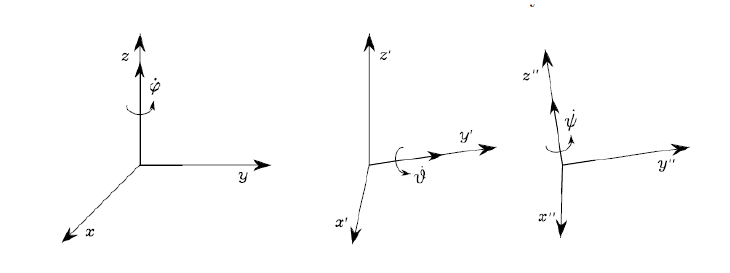
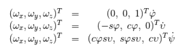
Then:
\bm{\omega}_e = \left( \begin{array}{ccc} 0 & -s\varphi & c\varphi s\upsilon \\ 0 & c\varphi & s\varphi s\upsilon \\ 1 & 0 & c\upsilon \\ \end{array} \right) \bm{\dot{\phi}}_e = \mathbf{T}(\bm{\phi}_e)\bm{\dot{\phi}}_e
And:
\mathbf{v}_e = \left( \begin{array}{c} \mathbf{\dot{p}}_e \\ \bm{\omega}_e \\ \end{array} \right) = \left( \begin{array}{cc} \mathbf{I} & \mathbf{0} \\ \mathbf{0} & \mathbf{T}(\bm{\phi}_e) \\ \end{array} \right)\left( \begin{array}{c} \mathbf{\dot{p}}_e \\ \bm{\dot{\phi}}_e \\ \end{array} \right) = \mathbf{T}_A(\bm{\phi}_e)\mathbf{\dot{x}}_e
Recalling that \mathbf{v}_e=\mathbf{J}(\mathbf{q})\mathbf{\dot{q}} and \mathbf{\dot{x}}_e=\mathbf{J}_A(\mathbf{q})\mathbf{\dot{q}}, the following relation between Jacobians is obtained:
\mathbf{J}(\mathbf{q})=\mathbf{T}_A(\bm{\phi}_e)\mathbf{J}_A(\mathbf{q})
Consider now the case of XYZ Euler angles:
\begin{array}{ccl} (\omega_x,\omega_y,\omega_z)^T &=& (1,\;0,\;0)^T \dot{\varphi}\nonumber\\ (\omega_x,\omega_y,\omega_z)^T &=& (0,\; c\varphi, \;s\varphi)^T\dot{\upsilon} \nonumber\\ (\omega_x,\omega_y,\omega_z)^T &=& (s\upsilon, \;-s\varphi c\upsilon, \;c\varphi c\upsilon)^T\dot{\psi} \nonumber \end{array}
\bm{\omega}_e = \left( \begin{array}{ccc} 1 & 0 & s\upsilon \\ 0 & c\varphi & -s\varphi s\upsilon \\ 0 & s\varphi & c\varphi c\upsilon \\ \end{array} \right)\bm{\dot{\phi}}_e = \mathbf{T}(\bm{\phi}_e)\bm{\dot{\phi}}_e
And for small angles, \mathbf{T}(\bm{\phi}_e)=\mathbf{I}_3.
Forces
The forces and moments at the end effector (\mathbf{h}_e) are related with the joint torques through the transpose of the Jacobian:
\bm{\tau} = \mathbf{J}^T(\mathbf{q})\mathbf{h}_e
- The range space of \mathbf{J}^T is composed of the joint torques that can balance the EE forces.
- The null space of \mathbf{J}^T is composed of the EE forces that do not require balancing of any joint torque (they are completely absorbed by the mechanical structure of the manipulator).
Using \mathbf{T}_A(\bm{\phi}_e), that relates \mathbf{v}_e and \mathbf{\dot{x}}_e, the following is defined:
\mathbf{h}_A = \mathbf{T}^T_A \mathbf{h}_e
Control issues
Dynamic model
The dynamic model of a manipulator is:
\mathbf{B}(\mathbf{q})\mathbf{\ddot{q}}+ \mathbf{C}(\mathbf{q},\mathbf{\dot{q}})\mathbf{\dot{q}}+\mathbf{F}\mathbf{\dot{q}}+\mathbf{g}(\mathbf{q})=\bm{\tau}
where:
- \mathbf{B}(\mathbf{q}) is the inertia matrix.
- \mathbf{C}(\mathbf{q},\mathbf{\dot{q}}) is the matrix of centrifugal and Coriolis terms.
- \mathbf{F} is the viscous friction matrix.
- \mathbf{g}(\mathbf{q}) is the gravitational term.
- \bm{\tau} is the applied vector of torques (or forces in the case of linear joints).
To control the motion of the manipulator in free space, the vector of torques \bm{\tau} has to be applied. This is done by the actuators through proper transmissions. In the absence of backslash in the actuators, the relationship between the actuated torque \bm{\tau}_m and the torque \bm{\tau} at the joints is:
\bm{\tau} = \mathbf{K}_r \bm{\tau}_m
with \mathbf{K}_r a diagonal matrix with values much greater than unity. The vector of actuated torques is proportional to the vector of armature currents \mathbf{i}_a:
\bm{\tau}_m = \mathbf{K}_t \mathbf{i}_a.
If current control drives are used, \mathbf{i}_a is proportional to the applied voltage \mathbf{v}_c:
\mathbf{i}_a = \mathbf{G}_i \mathbf{v}_c.
Therefore:
\bm{\tau} = \mathbf{K}_r \mathbf{K}_t \mathbf{G}_i \mathbf{v}_c.
Let \mathbf{u} be defined as:
\mathbf{u} = \mathbf{K}_r \mathbf{K}_t \mathbf{G}_i \mathbf{v}_c.
Then:
\mathbf{B}(\mathbf{q})\mathbf{\ddot{q}}+ \mathbf{C}(\mathbf{q},\mathbf{\dot{q}})\mathbf{\dot{q}}+\mathbf{F}\mathbf{\dot{q}}+\mathbf{g}(\mathbf{q})=\mathbf{u}
Lyapunov stability analysis
The Lyapunov Direct Method testes for stability without needing to solve the differential system equations.
If it is possible to associate an energy-based description with an autonomous dynamic system such that for each state of the system (except the equilibrium state) the time rate of such energy is negative, then energy decreases along any system trajectory until it attains its minimum at the equilibrium state.
Let V(\mathbf{e}) be a scalar function such that:
\begin{array}{ccc} V(\mathbf{e}) &>& 0 \;\;\forall \mathbf{e} \neq \mathbf{0} \\ V(\mathbf{e}) &=& 0 \;\; \mathbf{e}=\mathbf{0} \\ \dot{V}(\mathbf{e}) &<& 0 \;\; \forall \mathbf{e}\neq \mathbf{0} \\ V(\mathbf{e}) &\rightarrow& \infty \;\; \|e\|\rightarrow \infty \end{array}
The existence of such function ensures global asymptotic stability of the equilibrium state \mathbf{e}=\mathbf{0}.