Motion Control

The control problem

The different techniques and schemes for controlling the motion of a manipulator depend on several issues like:

• The goal: We may need to track a trajectory or simply to position the manipulator at a given configuration.
• The morphology of the robot: The kinematic and dynamic equations of a Cartesian robot are simpler to those of an anthropomorphic manipulator, and therefore the control schemes required differ.
• The driving system: Electric motors with reduction gears of high ratios make it possible to linearize and decouple the system dynamics (although friction and backslash may degrade the performance). On the other hand, direct drives have no backslash but suffer from non-linearities and coupling in the system dynamics.
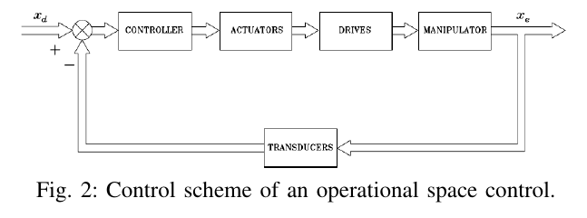
• Space where the control is done: Control in joint space (Fig. 1) requires first the inverse kinematics (IK) to transform from the operational space requirements \mathbf{x}_d to \mathbf{q}_d. Then, the control loop is responsible of making the actual motion \mathbf{q} to track the desired one \mathbf{q}_d. On the other hand, control in operational space (Fig. 2) has \mathbf{x}_d as input, i.e. the IK is embedded in the control loop.

In joint space the control scheme is simpler, but uncertainties in the structure are not absorbed by the feedback loop, since the IK is done in open loop, In operational space this disadvantage is overcome but the control scheme is more complex and, moreover, \mathbf{x}_e is not usually measured but computed from \mathbf{q}_e using the forward kinematics (FK).

Decentralized control vs. centralized control

Let \mathbf{q} and \mathbf{q}_m be the vectors of joint and actuator values, respectively, and \mathbf{\tau} and \mathbf{\tau}_m the corresponding torques. Let also \mathbf{K}_r be the n\times n diagonal matrix describing the reduction gears:

Then, the expressions of a velocity controlled driving system are:

Then (see Fig. 3 below):

Provided that the dynamics of the manipulator is given by:

the dynamics of the manipulator together with a drive modelled as a velocity-controlled generator results (see Fig. 4 below):

with

The following can be derived. If taking into account Eq.~(3):

1. gears with high reduction ratios are used (elements of \mathbf{K}_r \uparrow\uparrow),
2. high efficiency servomotors are used (elements of \mathbf{R}_a \downarrow\downarrow),
3. not high speeds and/or accelerations are required (required \mathbf{\tau} values \downarrow\downarrow).

Then \mathbf{G}_v \mathbf{v}_c - \mathbf{K}_v \mathbf{K}_r \mathbf{\dot{q}}_m \simeq 0, and:

Since \mathbf{G}_v^{-1} \mathbf{K}_v \mathbf{K}_r is a diagonal matrix, this means that the velocity of the i-th joint can be controlled by the i-th control voltage, i.e. a decentralized control structure can be used.

Otherwise, i.e. if large speeds/accelerations are required and, moreover, direct drives are used (\mathbf{K}_r = \mathbf{I}), then a decentralized control structure cannot be used. In this case, it is better to assure a driving system characterized by a current control (the actuator then behaves as a torque-controlled generator) in order to reduce the sensitivity to parameter variations (see expression of \mathbf{F} in Eq. (7)).

In this case \mathbf{i}_a = \mathbf{G}_i \mathbf{v}_c and (see Fig. 5 below):

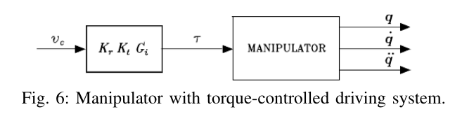
Then, the dynamics of the manipulator together with a drive modelled as a torque-controlled generator results (see Fig. 6 below):

with

In this case, a centralized control structure is required.

Control in joint space vs. control in operational space

Joint-space control assumes a desired trajectory in terms of joint values, i.e. \mathbf{q}_d, and the corresponding velocities and accelerations. Then, since motion specification is usually done in operational space, i.e. as \mathbf{x}_d, then an IK algorithm is required to transform operational space references into joint space references (the inversion of the firs-order and second-order differential kinematics is costly and usually substituted by numerical differentiation of \mathbf{q}_d).

If operational space control is used, the input is the desired trajectory in the operational space, the measured joint values are transformed using the FK, and the trajectory inversion is not required now, and simply substituted by a suitable coordinate transformation embedded in the feedback loop. However, the computational cost is higher and requires sampling times that may degrade the performance of the system. Therefore, control in operational space is left to applications where the environment constrains the robot motions and force/position control strategies, or visual control strategies, are required to properly control the task.

Two schemes are possible for operational space control:

1. Jacobian inverse control (Fig.7).
2. Jacobian transpose control (Fig. 8).

Decentralized control

The manipulator is considered as a set of n independent systems, each one controlled as a SISO system, and the couplings are treated as disturbances.

The dynamics of the manipulator can be rewritten in the variables \mathbf{q}_m and \mathbf{\tau}_m. Since \mathbf{q}_m = \mathbf{K}_r \mathbf{q} and \mathbf{\tau}_m = \mathbf{K}_r^{-1} \mathbf{\tau} it results:

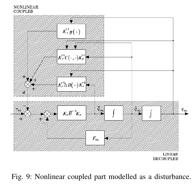
This expression can be simplified to (se Fig. 9 below):

with:

\overline{\mathbf{B}} is a diagonal matrix whose elements represent the resulting average inertia at each joint, whereas \Delta \mathbf{B}(\mathbf{q}) contains the configuration dependant terms (function of sine and cosine for revolute joints).

The \mathbf{d} signal can be considered a disturbance when:

• high gear reduction ratios are used (\mathbf{K}_r \uparrow\uparrow)
• there are low velocities and accelerations required.

Then, a decentralized control can be applied.

A position feedback scheme

We assume that the actuator is a rotary electric DC motor, with \mathbf{q}_m = \mathbf{\Theta}_m, as ahown in Fig. 10 below, where \mathbf{K}_t, \mathbf{R}_a, \mathbf{K}_v are the motor constants and \mathbf{I}_m is the average inertia reported to the motor axis.

Then, the position feedback scheme to drive control is shown in Fig. 11 below, where the torque disturbance \mathbf{D} has been transformed to voltage by factor \mathbf{R}_a/\mathbf{K}_t, \textbf{K}_{T\!P} is the position transducer constant and C_p(s) is a PI controller:

A PI controller allows to correctly reject disturbances:

• A high value of K_p reduces the effect of \mathbf{D}.
• The integral part forces a zero in the transfer function \frac{\Theta_m(s)}{D(s)} that allows the cancellation of gravity in the angular position in steady state.

The transfer functions with respect to the reference and to the disturbance are:

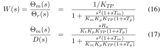
W(s) has one zero and three poles:

The root locus for T_p>>T_m is shown in Fig. 12 below.

For high values of K_p it results \frac{1}{\tau}\simeq \frac{1}{T_p} and the zero of W(s) tends to cancel the effects of the real pole.

The position feedback scheme can be extended to position-velocity feedback and to position-velocity-acceleration feedback, which allows more control parameters to tune the response.

Decentralized feed-forward compensation

Feed-forward (FF) terms can be introduced to improve the performance by reducing the tracking errors when high values of speed and acceleration are required (se Fig. 13 below).

If position feedback is substituted by position-velocity feedback or by position-velocity-acceleration feedback, the FF computation requires less knowledge of the model (i.e. T_m, K_m values).

Centralized feed-forward compensation

The idea is to add an extra term to the feed-forward compensation that is able to compensate the disturbance itself, rather than its effects, by taking advantage of the model knowledge. We had:

We can now define:

And then add an FF term \mathbf{R}_a\mathbf{K}_t^{-1}\mathbf{d}_d (see Fig. 14 below).

This centralized FF action:

• Compensates the nonlinear coupling due to the inertial, coriolis, centrifugal and gravitational terms that depend on the structure and that vary during the manipulator motion.
• Is computationally costly. This cost can be reduced if only the gravitational part \mathbf{K}_r^{-1}g(\mathbf{q}) and the diagonal terms of the inertial part \mathbf{K}_r^{-1} \Delta \mathbf{B}(\mathbf{q})\mathbf{K}_r^{-1} are computed.
• Tends to compensate the disturbance \mathbf{d} and allows the control system to operate in a better condition.

Centralized control

• If large speeds are required and/or direct-drive actuation is employed, the non-linear coupling terms have a great influence.
• It is advisable to design control schemes that take advantage of a detailed knowledge of the manipulator dynamics to compensate for the non-linear couplings, rather than trying to reduce their effect, i.e. to use centralized control schemes.
• The computed-torque centralized FF compensation presented in the previous section worked in this line, but it was computed on the desired trajectory; what it is proposed now is to use the dynamic model in the closed loop.

PD control with gravity compensation in the joint space

Consider a regulation problem where a fixed configuration \mathbf{q}_d is desired, the error is \tilde{\mathbf{q}} = \mathbf{q}_d - \mathbf{q}, and the dynamics of the manipulator is:

The system state is defined as [\tilde{\mathbf{q}}^T, \dot{\mathbf{q}}^T].

The question is to find which is the control law \mathbf{u} that brings the robot towards \mathbf{q}_d in an assimptotically stable manner.

The Lyapunov direct method can be used to determine such law. If a Lyapunov function V(\mathbf{q}, \dot{\mathbf{q}}) is formed such that \dot{V}(\mathbf{q}, \dot{\mathbf{q}}) < 0 along all the trajectories, then the system is assimptotically stable.

V(\mathbf{q}, \dot{\mathbf{q}}) is usually set as a function of the system energy. Let consider the following positive definite quadratic form:

with \mathbf{K}_P a n\times n positive definite matrix.

Differentiating w.r.t. time and recalling that \mathbf{q}_d is constant:

From the system dynamics:

Substituting this expression in Eq. (22), and taking into account that \mathbf{N}=\dot{\mathbf{B}} - 2\mathbf{C} is skewsymetric and therefore \dot{\mathbf{q}}^T\mathbf{N}\dot{\mathbf{q}}=0, we obtain:

If the control law \mathbf{u} = g(\mathbf{q}) + \mathbf{K}_P \tilde{\mathbf{q}} is chosen, it results:

and the system is assimptotically stable.

The control law has:

• Gravity compensation
• A proportional term

Then, a derivative term described by a positive definite matrix \mathbf{K}_D can be added that accelerates the convergence (see Fig. 15 below):

This results in a PD controller with gravity compensation.

In this case:

According to this, V decreases for all system trajectories, as long as \dot{\mathbf{q}}\neq 0.

The dynamics of the system with the PD controller is:

And at the equilibrium point (\dot{\mathbf{q}} = \ddot{\mathbf{q}} = 0) is simplified to \mathbf{K}_P \tilde{\mathbf{q}} = 0, i.e. the desired configuration is attained:

Any manipulator equilibrium posture is globally assimptotically stable under PD linear action with gravity compensation (being \mathbf{K}_P and \mathbf{K}_D positive definite matrices).

PD control with gravity compensation in the operational space

Consider a regulation problem where a fixed end effector pose \mathbf{x}_d is desired, the error is \tilde{\mathbf{x}} = \mathbf{x}_d - \mathbf{x}_e, and the dynamics of the manipulator is:

Let consider the following positive definite quadratic form:

with \mathbf{K}_P a n\times n positive definite matrix.

Its time derivative is:

Since a constant pose is desired, \dot{\mathbf{x}}_d=0, and hence \dot{\tilde{\mathbf{x}}} = \dot{\mathbf{x}}_d - \dot{\mathbf{x}}_e= - \dot{\mathbf{x}}_e = - \mathbf{J}_A(\mathbf{q}) \dot{\mathbf{q}}. Then the \dot{V} results:

From the system dynamics:

Substituting this expression in Eq. (32), we obtain:

If the control law \mathbf{u} = g(\mathbf{q}) + \mathbf{J}_A^T(\mathbf{q})\mathbf{K}_P \tilde{\mathbf{x}} is chosen, it results:

and the system is assimptotically stable.

As before, the control law has:

• Gravity compensation
• A proportional term

And also also as before, a derivative term described by a positive definite matrix \mathbf{K}_D can be added that accelerates the convergence (see Fig. 16 below):

This results in a PD controller with gravity compensation in the operational space.

In this case:

According to this, V decreases for all system trajectories, as long as \dot{\mathbf{q}}\neq 0.

The dynamics of the system with the PD controller is:

And at the equilibrium point (\dot{\mathbf{q}} = \ddot{\mathbf{q}} = 0) is simplified to \mathbf{J}_A^T(\mathbf{q})\mathbf{K}_P \tilde{\mathbf{x}} = 0, i.e. the desired pose is attained:

Final remark: Sometimes \mathbf{x}_e and \dot{\mathbf{x}}_e are directly measured; then the blocks k(\cdot) and \mathbf{J}_A(\mathbf{q}) in the block schema of Fig. 16 are not needed.

Inverse dynamics control in the joint space

Consider the tracking problem where the robot is desired to follow a given trajectory described by \mathbf{q}_d(t), \dot{\mathbf{q}}_d(t), and \ddot{\mathbf{q}}_d(t).

The dynamics of the manipulator is:

which can be rewritten as:

If we chose an input \mathbf{u} = \mathbf{B}(\mathbf{q}) \mathbf{y} + \mathbf{n}(\mathbf{q}, \mathbf{\dot{q}}), then the following linear dynamics appear:

where the \mathbf{y} is the new control input, i.e. a nonlinear state-feedback resulted in an input/output linearization of the system (see Fig. 17 below).

Now, the manipulator control problem has reduced to that of finding a stabilization control law \mathbf{y}. If we chose \mathbf{y} = -\mathbf{K}_P\mathbf{q} - \mathbf{K}_D\dot{\mathbf{q}} + \mathbf{r}, then the system dynamics \mathbf{\ddot{q}} = \mathbf{y} becomes \ddot{\mathbf{q}} + \mathbf{K}_D\dot{\mathbf{q}} + \mathbf{K}_P\mathbf{q} = \mathbf{r}, which is assimptotically stable for \mathbf{K}_P and \mathbf{K}_D positive definite.

If \mathbf{K}_P and \mathbf{K}_D are diagonal matrices, then the system is decoupled, i.e. reference r_i controls joint q_i.

This control scheme allows to solve tracking problems. Effectively, if we chose \mathbf{r}=\ddot{\mathbf{q}}_d+ \mathbf{K}_D\dot{\mathbf{q}}_d + \mathbf{K}_P\mathbf{q}_d then it results (see Fig. 18 below):

which expresses the dynamics of the error while tracking the specified trajectory.

Note:

• \mathbf{B}(\mathbf{q}) and \mathbf{n}(\mathbf{q}, \mathbf{\dot{q}}) are computed on-line. This is computationally costly. Therefore, sometimes only the dominant terms are computed.
• The approach is based on a perfect cancellation of the dynamics terms. This is difficult or even not possible if only the dominant terms are used, and therefore robust and adaptive methods are proposed:
• Robust control adds an additional term to counteract the effects of approximations.
• Adaptive control adapts the parameters of the model to the true values.