Visual Servoing

The visual servoing problem

Objective: To ensure that the end-effector reaches and keeps a desired pose w.r.t. an observed object. Objects are observed with a camera and the use of image processing (image segmentation plus image interpretation) that extracts image feature parameters.

The stated objective can be solved in two ways:

• The look-and-move approach uses visual measurements in open-loop. Therefore, it is sensitive to uncertainties like the possible poor position accuracy of the manipulator or the uncertainties in the actual location of the objects.
• The visual-servoing approach proposes the use of the visual measurements in closed-loop, i.e. visual measurements are fed back to the control to compute the appropriate command to achieve the goal.

As a difference with other feedback control schemes, visual-servoing has controlled variables not directly measured by a sensor but obtained through a computationally expensive process.

The visual-servoing problem depends on:

1. The position of the camera:

• eye-to-hand: camera fixed w.r.t. the world. Has fixed accuracy but problems of occlusion.
• eye-in-hand: camera held by the gripper. Solves occlusions problems but has variable accuracy (although not relevant when near the object).

2. Number of cameras:

• one-camera: Simple. Constrained to 2D vision.
• Two cameras: Allow stereo vision and the obtaining of 3D info.

3. Object motion:

• Fixed object: Regulation problem
• Moving object: Tracking problem.

4. Space where the control is done:

• Operational space: Requires the computation of the pose of the object and a position-based visual servoing scheme.

• Advantages: A desired time-response of the end-effector motion can be obtained by selecting the appropriate control parameters.
• Disadvantages: It requires the knowledge of the object, it is sensitive to camera calibration, and no direct control of the image parameters may lead the object to be outside the field of view.

• Image space: The control action is computed on the basis of the error between image feature parameters at the current configuration and the desired ones.

• Advantages: The real-time estimation of the object pose is not required, and the object is always kept inside the camera field of view.
• Disadvantages: Non-linearities in the mapping between the object features and the corresponding image parameters may lead to singularities.

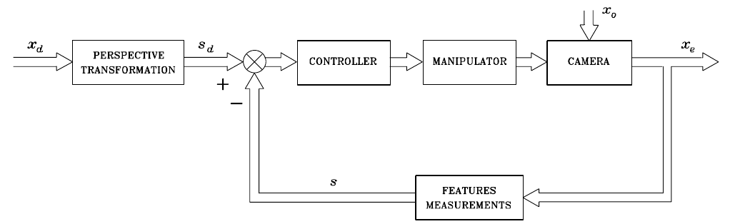
In this tutorial we will focus on position-based control schemes to solve the visual-servoing problem considering a single hand-held camera and fixed objects.

Pose Estimation

The feature vector

Let \{B\} be the world reference frame and \bm{T}_c^b be the transformation that defines the reference frame of a camera w.r.t. \{B\}.

If \bm{P}=[p_x,p_y,p_z]^T is a point and \tilde{\bm{p}}=[\bm{p}^T,1]^T its generalized representation, then the coordinates from the reference frame of the camera are:

\tilde{\bm{p}}^c = [p^c_x,p^c_y,p_z^c, 1]^T = \bm{T}_c^b \tilde{\bm{p}}

The perspective transformation of a camera with distance focus f leads to the following values:

\begin{aligned} \bm{X}_f &=& -f \frac{p_x^c}{p_z^c}\nonumber \\ \bm{Y}_f &=& -f \frac{p_y^c}{p_z^c},\label{eqXfYf}\end{aligned}

And considering a “virtual” image plane located at z_c=f and defining \bm{X} = \frac{p_x^c}{p_z^c} and \bm{Y} = \frac{p_y^c}{p_z^c}, the above expressions become:

\begin{aligned} \bm{X}_f &=& f \bm{X} \nonumber \\ \bm{Y}_f &=& f \bm{Y} \end{aligned}

The representation in the virtual image plane of point [\bm{X}_f,\bm{Y}_f] depends on the spatial sampling (the spatial sampling units are the pixels).

Pixel coordinates are obtained through a scaling process:

\begin{aligned} \bm{X}_I &=& f \alpha_x \bm{X} +\bm{X}_0 \nonumber \\ \bm{Y}_I &=& f \alpha_y \bm{Y} + \bm{Y}_0,\end{aligned}

with \bm{X}_0, and \bm{Y}_0, being the offsets of the origin in the pixel coordinate system. This can be expressed in matrix form as:

\left[\begin{array}{c} \bm{X}_I \\ \bm{Y}_I \\ 1 \end{array} \right] = \left[\begin{array}{ccc} f \alpha_x & 0 & \bm{X}_0 \\ 0 & f \alpha_y & \bm{Y}_0 \\ 0 & 0 & 1 \end{array} \right] \left[\begin{array}{c} \bm{X} \\ \bm{Y} \\ 1 \end{array} \right] = \Omega \left[\begin{array}{c} \bm{X} \\ \bm{Y} \\ 1 \end{array} \right]

The parameters (\alpha_x, \alpha_y, \bm{X}_0, \bm{Y}_0, f) are the intrinsic parameters of the camera, and are assumed to be known.

Then, we will work with the coordinates [\bm{X},\bm{Y}]^T which will be called normalized coordinates.

The relationship between these coordinates and the 3D coordinates of the point w.r.t. the camera frame can be expressed as:

\lambda \left[\begin{array}{c} \bm{X} \\ \bm{Y} \\ 1 \end{array} \right] = \Pi \left[\begin{array}{c} p_x^c \\ p_y^c \\ p_z^c \\ 1 \end{array} \right],

with:

\Pi = \left[\begin{array}{cccc} 1 & 0 & 0 & 0 \\ 0 & 1 & 0 & 0 \\ 0 & 0 & 1 & 0 \end{array} \right].

Then, the feature vector of a point will be defined as:

\bm{s}=[\bm{X},\bm{Y}]^T,

and its expression in generalized coordinates as:

\tilde{\bm{s}}=[\bm{X},\bm{Y}, 1]^T.

The expression relating the feature vector and the corresponding point in the object is:

\lambda \tilde{\bm{s}} = \Pi \tilde{\bm{p}}^c

The feature vector can be extended to a set of points:

\bm{s} = \left[\begin{array}{c} \bm{s}_1 \\ \vdots \\ \bm{s}_n \end{array} \right], \; \textrm{with} \;\bm{s}_i = \left[\begin{array}{c} \bm{X}_i \\ \bm{Y}_i \end{array} \right].

Analytic solution

Given a set of points in the object and the associated feature vector, find the pose of the object w.r.t. the camera, i.e. \bm{T}_o^c.

Consider the point \bm{P}_i on the object. Its coordinates in the camera frame are:

\tilde{\bm{r}}_{o,i}^c = \bm{T}_o^c \tilde{\bm{r}}_{o,i}^o

And the corresponding feature vector in the image plane is \bm{s}_i = [\bm{X}_i, \bm{Y}_i]^T, that is related with \tilde{\bm{r}}_{o,i}^o with the expression:

\lambda_i \tilde{\bm{s}}_i = \Pi \bm{T}_o^c \tilde{\bm{r}}_{o,i}^o

Considering n points, a systems of equations results:

\begin{aligned} \lambda_1 \tilde{\bm{s}}_1 & = &\Pi \bm{T}_o^c \tilde{\bm{r}}_{o,1}^o\nonumber \\ &\vdots&\nonumber \\ \lambda_n \tilde{\bm{s}}_n & = & \Pi \bm{T}_o^c \tilde{\bm{r}}_{o,n}^o,\end{aligned}

This system can be solved for the unknown elements of \bm{T}_o^c. This is a difficult issue with possibly multiple solutions, that depends on the number of points and on whether they are coplanar or not. In the case of coplanar points it is affordable with the following procedure:

1. Let \bm{S}(\cdot) represent the skew-symmetric matrix:

   \bm{S}([x,y,x]^T) = \left[\begin{array}{ccc} 0 & -z & y\\ z & 0 & -x \\ -y & x & 0 \end{array} \right]

Apply it to the feature vector:

\bm{S}(\tilde{\bm{s}}_i) = \left[\begin{array}{ccc} 0 & -1 & \bm{Y}_i\\ 1 & 0 & -\bm{X}_i \\ -\bm{Y}_i & \bm{X}_i & 0 \end{array} \right] \; \textrm{with} \;\tilde{\bm{s}}_i = \left[\begin{array}{c} \bm{X}_i \\ \bm{Y}_i \\ 1 \end{array} \right]

2. Multiply \bm{S}(\tilde{\bm{s}}_i) to both sides of \lambda_i \tilde{\bm{s}}_i = \Pi \bm{T}_o^c \tilde{\bm{r}}_{o,i}^o, i.e.:

   \bm{S}(\tilde{\bm{s}}_i)\lambda_i \tilde{\bm{s}}_i = \bm{S}(\tilde{\bm{s}}_i)\Pi \bm{T}_o^c \tilde{\bm{r}}_{o,i}^o \label{Eq:step2}

The left part is the zero vector:

\left[\begin{array}{ccc} 0 & -1 & \bm{Y}_i\\ 1 & 0 & -\bm{X}_i \\ -\bm{Y}_i & \bm{X}_i & 0 \end{array} \right] \left[\begin{array}{c} \lambda_i \bm{X}_i \\ \lambda_i \bm{Y}_i \\ \lambda_i \end{array} \right] = \left[\begin{array}{c} 0 \\ 0 \\ 0 \end{array} \right]

From the right part, let define \bm{H} as:

\begin{aligned} \bm{H} \!\!&=&\!\! \Pi \bm{T}_o^c \!\!=\!\! \left[\begin{array}{cccc} 1 & 0 & 0 & 0 \\ 0 & 1 & 0 & 0 \\ 0 & 0 & 1 & 0 \end{array} \right] \!\!\left[\begin{array}{cccc} \bm{r}_1 & \bm{r}_2 & \bm{r}_3 & \bm{o}_{c,o}^c \\ 0 & 0 & 0 & 1 \end{array} \right]\nonumber = \left[\begin{array}{cccc} \bm{r}_1 & \bm{r}_2 & \bm{r}_3 & \bm{o}_{c,o}^c \end{array} \right] \end{aligned}

3. Make the following simplification. Consider that all the points are in the plane z=0, i.e. \bm{r}_{o,i}^o = [r_{x,i}, r_{y,i},0]^T. Then take only the non-null components of the points, redefine \bm{H} as \bm{H} = [\bm{r}_1 \; \bm{r}_2\; \bm{o}_{c,o}^c], and rewrite the previous equations as:

\bm{0} = \bm{S}(\tilde{\bm{s}}) \bm{H} [r_{x,i}, \; r_{y,i}, \; 1]^T \label{Eq:step3}

4. This last equation can be rewritten as:

\bm{A}_i(\bm{s}_i)\bm{h} = \bm{0}

with:

• \bm{h} the 9\times 1 vector obtained by stacking the components of \bm{H}, i.e. \bm{h} = [\bm{r}_1, \bm{r}_2, \bm{o}_{c,o}^c]^T

• \bm{A}_i(\bm{s}_i) a 3\times 9 matrix:

  \bm{A}(\bm{s}_i) = [r_{x,i} \bm{S}(\tilde{\bm{s}}_i) \; \; r_{y,i}\bm{S}(\tilde{\bm{s}}_i)\;\; \bm{S}(\tilde{\bm{s}}_i)]

The rank of \bm{A}(\bm{s}_i) is at most two, which is the rank of \bm{S}(\tilde{\bm{s}}_i).

5. Consider 4 coplanar points, with no triplets of colinear points. Then the rank of:

\bm{A}(\bm{s}) = \left[\begin{array}{c} \bm{A}_1(\bm{s}_1)\\ \bm{A}_2(\bm{s}_2)\\ \bm{A}_3(\bm{s}_3)\\ \bm{A}_4(\bm{s}_4) \end{array}\right],

is eight and the system of equations \bm{A}(\bm{s}) \bm{h}=\bm{0} can be solved up to a scaling factor, i.e. if the solution is \xi\bm{h} = \xi[\bm{h}_1 \; \bm{h}_2 \; \bm{h}_3 ]^T, then:

\begin{aligned} \bm{r}_1 &=& \xi \bm{h}_1\nonumber\\ \bm{r}_2 &=& \xi \bm{h}_2\nonumber\\ \bm{o}_{c,o}^c &=& \xi \bm{h}_3\end{aligned}

and \xi is computed by imposing the unit norm constraint of vectors \bm{r}_1 and \bm{r}_2:

|\xi| = \frac{1}{\Vert \bm{h}_1 \Vert} = \frac{1}{\Vert \bm{h}_2 \Vert}

The sign is chosen such that the solution places the object in front of the camera.

Finally, \bm{r}_3 = \bm{r}_1\times \bm{r}_2.

Position-based visual-servoing

PD control with gravity compensation

The PD control with gravity compensation scheme can be used for the visual-servoing problem, with the a different error definition as that used in the motion control problem (see step 3 below), and with the pose estimation procedure needed to compute the pose of the end-effector from the image.

The block scheme shown is:

And the control law is:

\mathbf{u} = g(\mathbf{q}) + \mathbf{J}_{A_d}^T(\mathbf{q},\tilde{\mathbf{x}}) ( \mathbf{K}_P \tilde{\mathbf{x}} - \mathbf{K}_D \mathbf{J}_{A_d}(\mathbf{q},\tilde{\mathbf{x}})\dot{\mathbf{q}} ),

with

\bm{J}_{A_d}(\bm{q},\tilde{\bm{x}}) = \bm{T}_A^{-1}(\bm{\phi}_{d,e}) \left[ \begin{array}{cc} \bm{R}_d^T & \bm{0} \\ \bm{0} & \bm{R}_d^T \end{array} \right] \bm{J}(\bm{q}),

In visual-servoing this scheme is used because the natural reference frame to work with is that of the camera.

Assuming a fixed object and a desired object-camera transformation \bm{T}_o^d, the following steps should be iterativelly applied:

1. Use the pose estimation procedure explained in Section Pose Estimation to compute \bm{T}_o^c, i.e. the current pose of the object w.r.t. the camera frame.
2. Compute the transform between the desired pose of the robot and the current one:

\bm{T}_c^d = \bm{T}_o^d (\bm{T}_o^c)^{-1} = \left[\begin{array}{cc} \bm{R}_c^d & \bm{o}_{d,c}^d \nonumber \\ \bm{0} & 1 \end{array} \right]

3. Compute the error as:

\tilde{\bm{x}} = -\left[\begin{array}{c} \bm{o}_{d,c}^d \\ \bm{\phi}_{d,c} \end{array} \right]\label{Eq-error}

with \bm{\phi}_{d,c} being the XYZ Euler angles representing \bm{R}_c^d. (remark that \tilde{\bm{x}} is not obtained directly from \tilde{\bm{x}}_{c,o} and \tilde{\bm{x}}_{d,o}).

4. Compute the analytical Jacobian \bm{J}_{A_d} (\bm{q},\tilde{\bm{x}}).
5. Apply the control command \bm{u}:

\mathbf{u} = g(\mathbf{q}) + \mathbf{J}_{A_d}^T(\mathbf{q},\tilde{\mathbf{x}}) ( \mathbf{K}_P \tilde{\mathbf{x}} - \mathbf{K}_D \mathbf{J}_{A_d}(\mathbf{q},\tilde{\mathbf{x}})\dot{\mathbf{q}} ),

With \bm{K}_P and \bm{K}_D positive definite the error \tilde{\bm{x}} is brought assimptotically to zero.

Resolved velocity control

The pose estimation procedure is computationally costly and therefore the visual information has to be processed with low frequency (usually one order of magnitude less than the one used in motion control). Due to this low frequency (i.e. large sampling time):

1. Low gains are required to guarantee stability.
2. The performance in terms of disturbance rejection is low.
3. The performance in terms of speed of convergence is low.

Then, to overcome these drawbacks, an alternative is:

1. To consider the manipulator equipped with a high-gain motion controller, i.e. consider it an ideal positioning device (\bm{q}(t) \simeq \bm{q}_r(t), where \bm{q}_r(t) is the reference trajectory).
2. To use the visual servoing to compute \bm{q}_r(t).

This way, visual servoing is achieved by computing the trajectory \bm{q}_r(t) on the basis of visual measurements, so that the operational space tracking error goes asymptotically to zero. The time derivative of this error is:

\dot{\tilde{\bm{x}}} = -\bm{J}_{A_d}(\bm{q},\tilde{\bm{x}}) \dot{\bm{q}} \label{Eq-xtildedot}

Then, this suggests the following choice for the joint space reference velocity (see Figure above):

\dot{\bm{q}}_r = \bm{J}_{A_d}^{-1}(\bm{q},\tilde{\bm{x}}) \bm{K} \tilde{\bm{x}}

which replaced in the Equation of \dot{\tilde{\bm{x}}} and considering \bm{q}(t) \simeq \bm{q}_r(t) yields to the linear equation:

\dot{\tilde{\bm{x}}} + \bm{K} \tilde{\bm{x}} = 0.

This equality, for a positive definite matrix K, implies that the operational space error tends to zero asymptotically with a convergence of exponential type and speed depending on the eigenvalues of matrix K; the larger the eigenvalues, the faster the convergence.

The above scheme is termed resolved-velocity control in the operational space, because it is based on the computation of velocity \dot{\bm{q}}_r from the operational space error. Trajectory \bm{q}_r(t) is then computed via a simple integration.

If \bm{K} is a diagonal matrix with the same gains for the positional part, the origin of the camera frame follows the line segment connecting the initial position to the desired position. On the other hand, the orientation trajectory depends on the particular choice of Euler angles used to define the orientation error. The possibility of knowing in advance the trajectory of the camera is important because, during the motion, the object may exit from the camera field of view, making visual measurements unavailable.