Rigid bodies and homogeneous transformations
Based on Sections 2.1-2.7 of Robotics: Modelling, Planning and Control .
Link to the practical session on Basic commands for representing position and orientation
Pose of a rigid object
Pose = position and orientation.
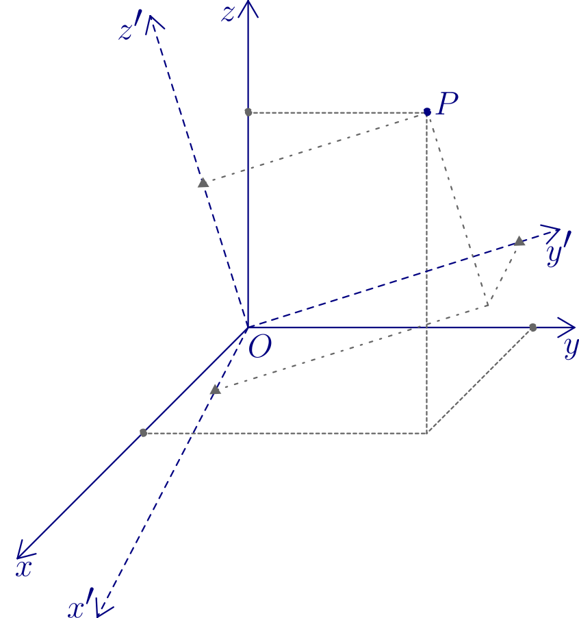
The pose of a rigid body is given by the position and orientation of a frame attached to it with respect to another reference frame:
\[\begin{split}\quad
\text{Position:}\;
\boldsymbol{o}' =
\begin{bmatrix}
o_x' \\
o_y' \\
o_z'
\end{bmatrix}
\quad
\text{Orientation:}
\quad
\left.
\begin{array}{l}
\boldsymbol{x}' = {x}'_x\,\boldsymbol{x} + {x}'_y\,\boldsymbol{y} + {x}'_z\,\boldsymbol{z} \\
\boldsymbol{y}' = {y}'_x\,\boldsymbol{y} + {y}'_y\,\boldsymbol{y} + {y}'_z\,\boldsymbol{z} \\
\boldsymbol{z}' = {z}'_x\,\boldsymbol{x} + {z}'_y\,\boldsymbol{y} + {z}'_z\,\boldsymbol{z}
\end{array}
\right\}
\quad
\text{Object frame axis w.r.t. reference frame}\end{split}\]
The components of each unit vector (e.g., \(\boldsymbol{x}' = [x_x', x_y', x_z']^T\) ) are the direction cosines of the frame of the object w.r.t. the reference frame.
Rotation Matrix
By adopting a compact notation, the three unit vectors describing the body orientation with respect to the reference frame can be combined in the
\((3 \times 3)\) matrix:
\[\begin{split}\boldsymbol{R} \; = \; \left[\boldsymbol{x}', \boldsymbol{y}', \boldsymbol{z}'\right] \; =\! \!
\quad
\begin{bmatrix}
{x}'_x && {y}'_x && {z}'_x\\
{x}'_y && {y}'_y && {z}'_y\\
{x}'_z && {y}'_z && {z}'_z
\end{bmatrix}\\\end{split}\]
Column vectors are orthogonal and have unit norm:
\[ \begin{align}\begin{aligned}\boldsymbol{x}^{'\,T} . \boldsymbol{y}' = 0 \quad
\boldsymbol{y}^{'\,T} . \boldsymbol{z}' = 0 \quad
\boldsymbol{z}^{'\,T} . \boldsymbol{x}' = 0\\\boldsymbol{x}^{'\,T} . \boldsymbol{x}' = 1 \quad
\boldsymbol{y}^{'\,T} . \boldsymbol{y}' = 1 \quad
\boldsymbol{z}^{'\,T} . \boldsymbol{z}' = 1\end{aligned}\end{align} \]
\(\boldsymbol{R}\) is an orthogonal matrix:
\[\begin{split}\boldsymbol{R}^{T} \: \boldsymbol{R} = \boldsymbol{I}_3 \\\end{split}\]
It follows, that \(\boldsymbol{R}^{T} = \boldsymbol{R}^{-1}\) and that \(det(\boldsymbol{R}) = 1\) (assuming the frame is right - handed).
This matrix satisfies: \(\boldsymbol{R} \: \in \: SO(3)\) , the special orthogonal group of \((3 \times 3)\) matrices with orthogonal columns and determinant equal to 1.
There are three equivalent geometric meanings of \(\boldsymbol{R}\) :
Elementary rotation
Representation of a vector
Rotation of a vector
a) Elementary Rotations:
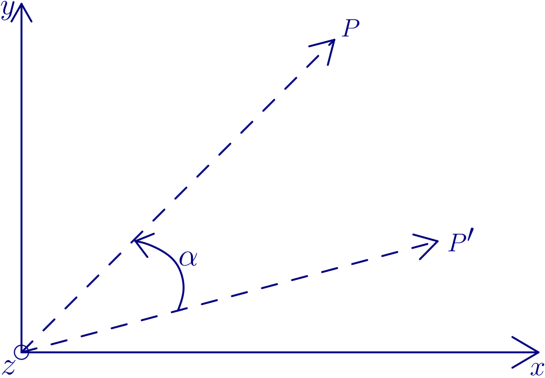
Rotations about one of the coordinate axes, e.g., the rotation about the \(z\) axis is:
\[\begin{split}\boldsymbol{R}_z(\alpha) =
\begin{bmatrix}
\cos(\alpha) & -\sin(\alpha) & 0 \\
\sin(\alpha) & \cos(\alpha) & 0 \\
0 & 0 & 1
\end{bmatrix}\end{split}\]
where the column represent the vectors of the new frame \(O\!\!-\!x'y'z'\) with respect to the reference frame \(O\!\!-\!xyz\) .
Analogously:
\[\begin{split}\boldsymbol{R}_y(\beta) = \quad
\begin{bmatrix}
cos(\beta) && 0 && sin(\beta)\\
0 && 1 && 0\\
-sin(\beta) && 0 && cos(\beta)
\end{bmatrix}\\
\\
\boldsymbol{R}_x(\gamma) = \quad
\begin{bmatrix}
1 && 0 && 0\\
0 && cos(\gamma) && -sin(\gamma)\\
0 && sin(\gamma) && cos(\gamma)
\end{bmatrix}\\\end{split}\]
This property holds: \(\;\boldsymbol{R}_{k}(-\theta) = \boldsymbol{R}_{k}^T(\theta)\; \text{for}\; k = x,y,z\) .
These matrices will be useful to describe rotations about an arbitrary axis in space.
\(\boldsymbol{R}\) describes the rotation about an axis in space needed to align the axis of the reference frame with the corresponding axis of the body frame.
b) Representation of a Vector:
Consider two frames with the same origin \(\; O\!\!-\!xyz\;\) and \(\;O\!\!-\!x'y'z'\) .
The coordinates of point P are:
\[\begin{split}\begin{aligned}
\boldsymbol{p} &= \left[p_{x}\;p_{y}\;p_{z}\right]^T\; \text{ w.r.t }\; O\!\!-\!xyz \\
\boldsymbol{p'} &= \left[p'_{x}\;p'_{y}\;p'_{z}\right]^T\; \text{ w.r.t }\; O\!\!-\!x'y'z'
\end{aligned}\end{split}\]
The relation is:
\[\boldsymbol{p} = p'_{x}\boldsymbol{x}'+p'_{y}\boldsymbol{y}'+p'_{z}\boldsymbol{z}'= \left[\boldsymbol{x}'\boldsymbol{y}'\boldsymbol{z}'\right]\boldsymbol{p'} = \boldsymbol{R} \boldsymbol{p'}\]
\(\boldsymbol{R}\) represents the transformation matrix of a vector in \(\;O\!\!-\!x'y'z'\:\) coordinates into the \(\;O\!\!-\!xyz\:\) coordinates.
The inverse transformation holds: \(\;\boldsymbol{p'} = \boldsymbol{R}^T\boldsymbol{p}\) .
c) Rotation of a vector
\(\boldsymbol{R}\) can be also seen as a matrix operator allowing rotation of a vector about a given axis.
\[\begin{split}\begin{aligned}
\boldsymbol{p'} &= \text{ vector in frame }\; O\!\!-\!xyz \\
\boldsymbol{p} &= \boldsymbol{R}\boldsymbol{p'} = \text{ rotated vector in frame }\;O\!\!-\!xyz
\end{aligned}\end{split}\]
Composition of Matrices
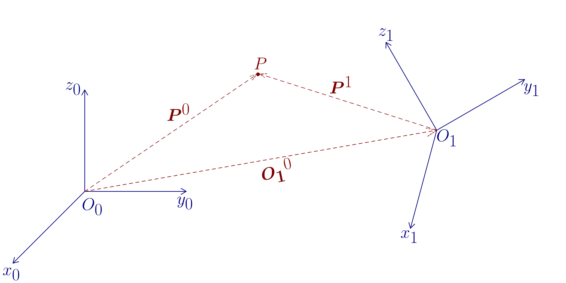
Consider:
\[\begin{split}\begin{aligned}
\boldsymbol{p}^0 &= \text{ point P w.r.t. }\; O\!\!-\!x_{0}y_{0}z_{0} \\
\boldsymbol{p}^1 &= \text{ point P w.r.t. }\; O\!\!-\!x_{1}y_{1}z_{1} \\
\boldsymbol{p}^2 &= \text{ point P w.r.t. }\; O\!\!-\!x_{2}y_{2}z_{2} \\
\boldsymbol{R}_{i}^j &= \text{Rotation of matrix of frame}\; i \text{ w.r.t. frame}\; j
\end{aligned}\end{split}\]
Then: \(\; \boldsymbol{p}^1 = \boldsymbol{R}_{2}^1\,\boldsymbol{p}^2\:\) (see (b) above)
Also:
\[\begin{split}\left.
\begin{aligned}
\boldsymbol{p}^0 &= \boldsymbol{R}_{1}^0\,\boldsymbol{p}^1 = \boldsymbol{R}_{1}^0\,\boldsymbol{R}_{2}^1\,\boldsymbol{p}^2\\
\boldsymbol{p}^0 &= \boldsymbol{R}_{2}^0\,\boldsymbol{p}^2
\end{aligned}
\right\}
\quad
\boldsymbol{R}_{2}^0 = \boldsymbol{R}_{1}^0 \,\boldsymbol{R}_{2}^1\end{split}\]
This can be interpreted as follows. Starting from \(\;O\!\!-\!x_{0}y_{0}z_{0}\:\) :
Rotate the frame according to \(\boldsymbol{R}_{1}^0\) to align it with \(O\!\!-\!x_{1}y_{1}z_{1}\) .
Rotate the frame (now aligned with \(O\!\!-\!x_{1}y_{1}z_{1}\) ) according to \(O\!\!-\!x_{1}y_{1}z_{1}\) so as to align it with \(O\!\!-\!x_{2}y_{2}z_{2}\) .
Important
These are rotations done about an axis of the current frame , then the composition of matrices is obtained by post multiplication .
\[\boldsymbol{R}_{2}^0 = \boldsymbol{R}_{1}^0 \,\boldsymbol{R}_{2}^1\]
When rotations are done about the axis of the fixed frame , then the computations of the matrices is obtained by premultiplication .
\[\boldsymbol{\bar{\boldsymbol{R}}_{2}^0 = \bar{\boldsymbol{R}}_{2}^1 \,R_{1}^0}\]
(\(\bar{\boldsymbol{R}}_{2}^1\) changes from 1 to 2 by a rotation around an axis of the fixed frame 0).
Euler Angles
Euler angles give a minimal representation of a rotation, i.e., only 3 parameters are used:
\[\boldsymbol{\phi} = \left[ \varphi, \; \theta, \; \psi \right]^T\]
Any generic rotation can be set as a composition of three elementary rotations (considering no consecutive rotations made about parallel axes) .
There are 12 sets of Euler angles. The most used are:
ZYZ (considering rotations about current frames)
RPY (Roll Pitch Yaw - considering rotations about fixed frame)
a) ZYZ
\(\boldsymbol{R}\) is obtained by the following consecutive elementary rotations about the ZYZ axes of the current frames :
\[\begin{split}\left.
\begin{aligned}
1. &\quad \boldsymbol{R}_{z}(\varphi) \\
2. &\quad \boldsymbol{R}_{y'}(\theta) \\
3. &\quad \boldsymbol{R}_{z''}(\psi) \\
\end{aligned}
\right\}\end{split}\]
Then:
\[\begin{split}\boldsymbol{R} = \overbrace{\boldsymbol{R}_{z}(\varphi)\;\boldsymbol{R}_{y'}(\theta)\;\boldsymbol{R}_{z''}(\psi)}^{\text{postmultiplication}} \;=
\quad
\begin{bmatrix}
c_\varphi c_\theta c_\psi - s_\varphi s_\psi & -c_\varphi c_\theta s_\psi - s_\varphi c_\psi & c_\varphi s_\theta \\
s_\varphi c_\theta c_\psi + c_\varphi s_\psi & -s_\varphi c_\theta s_\psi + c_\varphi c_\psi & s_\varphi s_\theta \\
-s_\theta c_\psi & s_\theta s_\psi & c_\theta
\end{bmatrix}\\\end{split}\]
The inverse problem is:
\[\begin{split}\text{Given }\boldsymbol{R} =
\begin{bmatrix}
r_{11} && r_{12} && r_{13}\\
r_{21} && r_{22} && r_{23}\\
r_{31} && r_{32} && r_{33}
\end{bmatrix}\;\;
\text{the Euler angles can be computed as: }
\left.
\begin{aligned}
\varphi &= \textrm{atan2} (r_{23},r_{13}) \\
\theta &= \textrm{atan2} (\sqrt{r_{13}^2+r_{23}^2},r_{33}) \\
\psi &= \textrm{atan2} (r_{32},-r_{31})
\end{aligned}
\right\}\end{split}\]
b) RPY angles
\[\boldsymbol{\phi} = \left[ roll, \; pitch, \; yaw \right]^T = \left[\varphi, \; \theta, \; \psi \right]^T\]
\(\boldsymbol{R}\) is obtained by the following consecutive elementary rotations about the XYZ axes of the fixed frame :
\[\begin{split}\left.
\begin{aligned}
(yaw)\; &1. \quad R_{x}(\psi) \\
(pitch)\; &2. \quad R_{y}(\theta) \\
(roll)\; &3. \quad R_{z}(\varphi) \\
\end{aligned}
\right\}\end{split}\]
Then:
\[\begin{split}\boldsymbol{R} = \overbrace{R_{z}(\varphi)\;R_{y}(\theta)\;R_{x}(\psi)}^{\text{premultiplication}} \;=
\quad
\begin{bmatrix}
c_\varphi c_\theta & c_\varphi s_\theta s_\psi - s_\varphi c_\psi & c_\varphi s_\theta c_\psi + s_\varphi s_\psi \\
s_\varphi c_\theta & s_\varphi s_\theta s_\psi + c_\varphi c_\psi & s_\varphi s_\theta c_\psi - c_\varphi s_\psi \\
-s_\theta & c_\theta s_\psi & c_\theta c_\psi
\end{bmatrix}\\\end{split}\]
The inverse problem is:
\[\begin{split}\text{Given }\boldsymbol{R} =
\begin{bmatrix}
r_{11} && r_{12} && r_{13}\\
r_{21} && r_{22} && r_{23}\\
r_{31} && r_{32} && r_{33}
\end{bmatrix}\;\;
\text{the RPY angles are: }
\left.
\begin{aligned}
\varphi &= \textrm{atan2} (r_{21},r_{11}) \\
\theta &= \textrm{atan2} (-r_{31},\sqrt{r_{32}^2+r_{33}^2}) \\
\psi &= \textrm{atan2} (r_{32},r_{33})
\end{aligned}
\right\}\end{split}\]
(angles in the range \(\left[\frac{-\pi}{2},\frac{\pi}{2}\right]\) ; different expressions for the range \(\left[\frac{\pi}{2},\frac{3\pi}{2}\right]\) )
Angle and Axis Representation
Non-minimal representation that uses 4 parameters:
\[\begin{split}\quad
\left\{
\begin{aligned}
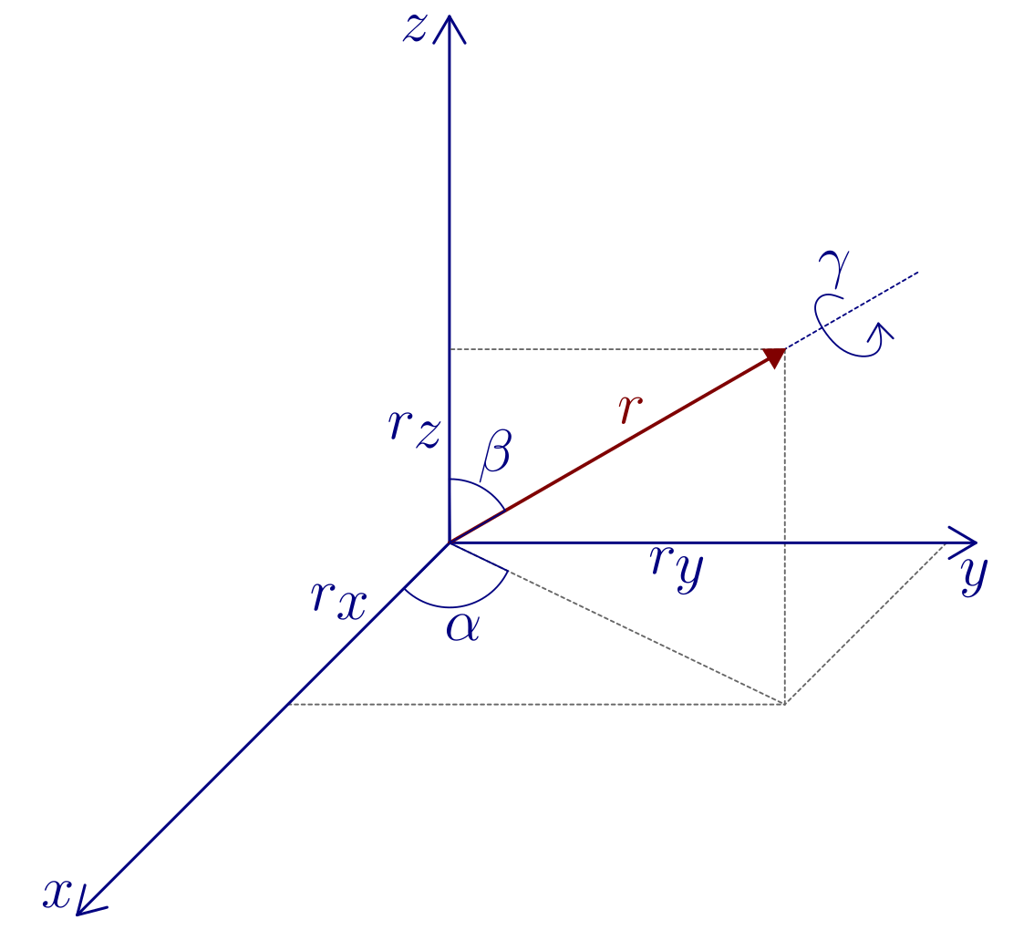
\boldsymbol{r} &= \left[r_{x}\;r_{y}\;r_{z}\right]^T = \text{vector}\\
\gamma &= \text{angle}
\end{aligned}
\right.\end{split}\]
Expresses the rotation of angle \(\gamma\) about axis \(\boldsymbol{r}\) (positive = counter clockwise).
\[\boldsymbol{R}(\gamma, \boldsymbol{r}) = \boldsymbol{R}_{z}(\alpha)\boldsymbol{R}_{y}(\beta)\boldsymbol{R}_{z}(\gamma)\boldsymbol{R}_{y}(-\beta)\boldsymbol{R}_{z}(-\alpha)\]
The inverse problem is:
\[\begin{split}\text{Given }\boldsymbol{R} =
\begin{bmatrix}
r_{11} && r_{12} && r_{13}\\
r_{21} && r_{22} && r_{23}\\
r_{31} && r_{32} && r_{33}
\end{bmatrix}\;\;
\text{The axis, angle representation is: }
\left.
\begin{aligned}
\boldsymbol{r} &= \frac{1}{2\,sin(\gamma)}
\begin{bmatrix}
r_{32} - r_{23}\\
r_{13} - r_{31}\\
r_{21} - r_{12}
\end{bmatrix}\\
\gamma &= {cos}^{-1}\left[\frac{r_{11}+r_{22}+r_{33}-1}{2}\right]
\end{aligned}
\right\}\end{split}\]
Quaternion
Also a non-minimal representation of four parameters, which is related to the axis-angle representation:
\[Q = \{ \eta, \boldsymbol{\epsilon} \} \quad \text{where:}\]
\[\begin{split}\left.
\begin{matrix}
\text{Scalar part} \quad \eta = \cos \frac{\gamma}{2} \\
\text{Vector part} \quad \boldsymbol{\epsilon} = \boldsymbol{r} \sin \frac{\gamma}{2}
\end{matrix}
\right\}\end{split}\]
The inverse problem is:
\[\begin{split}\text{Given } \boldsymbol{R} =
\begin{bmatrix}
r_{11} & r_{12} & r_{13} \\
r_{21} & r_{22} & r_{23} \\
r_{31} & r_{32} & r_{33}
\end{bmatrix}\;\;
\text{The quaternion is: }
\left.
\begin{aligned}
\eta &= \frac{1}{2} \sqrt{r_{11} + r_{22} + r_{33} - 1}\\
\boldsymbol{\epsilon} &= \frac{1}{2} \begin{bmatrix}
\textrm{sgn} (r_{23} - r_{23}) \sqrt{r_{11} - r_{22} - r_{33} + 1} \\
\textrm{sgn} (r_{13} - r_{31}) \sqrt{r_{22} - r_{11} - r_{33} + 1} \\
\textrm{sgn} (r_{21} - r_{12}) \sqrt{r_{33} - r_{11} - r_{22} + 1}
\end{bmatrix}
\end{aligned}
\right\}\end{split}\]
Note that the quaternion corresponding to \(R^{-1}\) is \(Q^{-1} = \{ \eta, - \boldsymbol{\epsilon} \}\) .