Lagrange formulation

Based on Section 7.1 of Robotics: Modelling, Planning and Control.

Link to the practical session on Dynamics

Introduction

The dynamics gives us the relationships between the joint torques and the motion of the structure.

• The direct dynamics problem:

  It is the problem of determining, for \(t > t_0\), the joint accelerations \(\boldsymbol{\ddot{q}}(t)\), and thus \(\boldsymbol{\dot{q}}(t)\) and \(\boldsymbol{q}(t)\), resulting from the joint torque \(\boldsymbol{\tau}(t)\) (and possibly end-effector contact forces \(\boldsymbol{h_e}\)), given an initial state of the system \(\boldsymbol{q}(t_0), \boldsymbol{\dot{q}}(t_0)\).

  \(\Rightarrow\) used in SIMULATION.

• The inverse dynamic problem:

  It is the problem of determining the joint torque \(\boldsymbol{\tau}(t)\) which are needed to generate a motion specified by the joint accelerations \(\boldsymbol{\ddot{q}}(t)\), velocities \(\boldsymbol{\dot{q}}(t)\) and positions \(\boldsymbol{q}(t)\), once the possible EE forces \(\boldsymbol{h_e}(t)\) are known.

  \(\Rightarrow\) used in PLANNING and CONTROL.

To solve the dynamic problems, the dynamic model of the manipulator is required, which can be obtained:

1. Using the Langrange formulation, which is simple and systematic.

2. Using the Newton-Euler formulation, which yields a recursive form that is computationally efficient.

In this tutorials, the Lagrange formulation will be used.

The Lagrange formulation

The Lagrange formulation is a systematic way to derive the dynamics of a mechanical structure, which is independent of the coordinate frames.

It is based on:

\[\begin{split}\left. \begin{array}{l} \text{1. The kinetic energy } {\cal T} \\ \text{2. The potential energy } {\cal U} \end{array} \right\} \quad \text{through the Lagrangian } {\cal L = T - U}\end{split}\]

Let:

• \(q_i, \, i = 1 \cdots n \;\) be the generalized coordinate (joint variables)

• \(\xi_i, \, i = 1 \cdots m \;\) be the force associated to \(q_i\) (joint torques).

Then, the Lagrangian equations are:

\[\frac{d}{dt} \left( \frac{\partial{\cal L}}{\partial \dot{{q}}_i} \right) - \frac{\partial {\cal L}}{\partial {q}}_i = \xi_i, \quad i = 1 \cdots n,\]

or in a compact form:

\[\frac{d}{dt} \left( \frac{\partial {\cal L}}{\partial {\boldsymbol{\dot{q}}}} \right)^T - \left( \frac{\partial {\cal L}}{\partial {\boldsymbol{q}}} \right)^T = \boldsymbol{\xi}\]

where:

\(\boldsymbol{\dot{q}} = [\dot{q_1}, \ldots, \dot{q_n}]^T\)

\(\boldsymbol{q} = [q_1, \ldots, q_n]^T\)

\(\boldsymbol{{\xi}} = [\xi_1, \ldots, \xi_n]^T\)

(recall that the derivative w.r.t. a column vector is a row vector)

An example

As a first example consider a 1-D manipulator (pendulum)

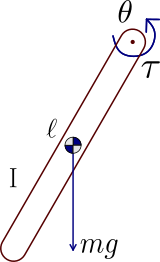
• The kinetic energy is \(\;{\cal T} = \frac{1}{2} I \dot{\theta}^2\)

• The potential energy is \(\;{\cal U} = mgl(1 - \cos\theta)\)

• The Lagrangian is \(\;{\cal L} = {\cal T} - {\cal U} = \frac{1}{2} I \dot{\theta}^2 - mgl(1 - \cos\theta)\)

• The torque is \(\;\xi = \tau - F\dot{\theta}\), where \(\tau\) is the actuation torque and \(F\) the viscous friction coefficient

Finally, the equation of motion is:

\[\frac{d}{dt} \left( \frac{\partial {\cal L}}{\partial \dot{\theta}} \right) - \frac{\partial {\cal L}}{\partial \theta} = \xi\]

\[I \ddot{\theta} + mgl \sin\theta = \tau - F\dot{\theta}\]

\[\boxed{ I \ddot{\theta} + F\dot{\theta} + mgl \sin\theta = \tau }\]

We will consider now a \(n\)-DOF manipulator. In the next subsections we will compute:

1. Kinetic energy

2. Potential energy

3. Equations of motion

Kinetic energy

The total kinetic energy a \(n\)-DOF manipulator is obtained by summing the kinetic energy of each link:

\[T = \sum_{i=1}^{n} T_{l_i}\]

where \(T_{l_i}\) denotes the kinetic energy of link \(i\).

In the following, we derive the kinetic energy of a single link.

Nomenclature

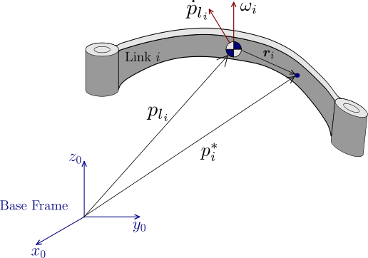
\(\boldsymbol{p_i^*} \, \equiv\) position vector of an elementary particle

\(\boldsymbol{p_{l_i}} \, \equiv\) position vector of the centre of mass

\[\begin{split}\boldsymbol{p_{l_i}} = \frac{1}{m_{l_i}} \int_{V_{l_i}} \boldsymbol{p_i^*} \, \rho \, dV \quad \left\{ \begin{align} \rho \, &\equiv \text{density} \\ V_{l_i} \, &\equiv \text{volume of link }i \\ m_{l_i}\, &\equiv \text{mass of link }i \end{align} \right.\end{split}\]

\[\boldsymbol{r_i} = \boldsymbol{p_i^*} - \boldsymbol{p_{l_i}} = \begin{bmatrix} r_{x_i}, r_{y_i}, r_{z_i} \end{bmatrix}^T\]

\(\boldsymbol{\dot{p}_i^*} \, \equiv\) velocity of an elementary particle

\(\boldsymbol{\dot{p}_{l_i}} \, \equiv\) linear velocity of the centre of mass

\(\boldsymbol{\omega_i} \, \equiv\) angular velocity of link \(i\) w.r.t. the base frame, \(\boldsymbol{\omega}_i = [\omega_x \,\; \omega_y \,\; \omega_z]^T\)

Velocity of an elementary particle

The velocity of an elementary particle as a function of the linear velocity of the centre of mass and the angular velocity of link is:

\[\boldsymbol{\dot{p}_i^*} = \boldsymbol{\dot{p}_{l_i}} + \boldsymbol{\omega}_i \times \boldsymbol{r}_i \,\:\]

This expression can be simplified using the skew-symmetric operator \(S(\cdot)\).

\[\begin{split}S(\boldsymbol{\omega}_i) = \begin{bmatrix} 0 & -\omega_z & \omega_y \\ \omega_z & 0 & -\omega_x \\ -\omega_y & \omega_x & 0 \end{bmatrix}\end{split}\]

\[\boldsymbol{\dot{p}_i^*} = \boldsymbol{\dot{p}_{l_i}} + S(\boldsymbol{\omega}_i)\boldsymbol{r}_i \:\:\]

Kinetic energy of a link

Then, the kinetic energy of link \(i\) is:

\[T_{l_i} = \frac{1}{2} \int_{V_{l_i}} \boldsymbol{\dot{p}_i}^{T} \boldsymbol{\dot{p}_i}^* \rho dV\]

\[= \frac{1}{2} \int_{V_{l_i}} (\boldsymbol{\dot{p}}_{l_i} + S(\boldsymbol{\omega}_i)\boldsymbol{r}_i)^T (\boldsymbol{\dot{p}}_{l_i} + S(\boldsymbol{\omega}_i)\boldsymbol{r}_i) \rho dV\]

\[= \frac{1}{2} \int_{V_{l_i}} \boldsymbol{\dot{p}}_{l_i}^T \boldsymbol{\dot{p}}_{l_i} \rho dV + \frac{1}{2} \int_{V_{l_i}} 2\boldsymbol{\dot{p}}_{l_i}^T S(\boldsymbol{\omega}_i)\boldsymbol{r}_i \rho dV + \frac{1}{2} \int_{V_{l_i}} (S(\boldsymbol{\omega}_i)\boldsymbol{r}_i)^T (S(\boldsymbol{\omega}_i)\boldsymbol{r}_i) \rho dV\]

There are three terms:

1. A pure translational part

2. A mutual part, i.e. translational and rotational

3. A pure rotational part

The expressions of these parts can be simplified as follows:

1. Translational part:

\[\frac{1}{2} \int_{V_{l_i}} \boldsymbol{\dot{p}}_{l_i}^T \boldsymbol{\dot{p}}_{l_i} \rho dV=\frac{1}{2} m_{l_i} \boldsymbol{\dot{p}}_{l_i}^T \boldsymbol{\dot{p}}_{l_i}\]

2. Mutual part:

\[\frac{1}{2} \int_{V_{l_i}} 2\boldsymbol{\dot{p}}_{l_i}^T S(\boldsymbol{\omega}_i)\boldsymbol{r}_i \rho dV=\boldsymbol{\dot{p}}_{l_i}^T S(\boldsymbol{\omega}_i) \int_{V_{l_i}} (\boldsymbol{p}_i^* - \boldsymbol{p}_{l_i}) \rho dV = \boldsymbol{\dot{p}}_{l_i}^T S(\boldsymbol{\omega}_i) \left[ \int_{V_{l_i}} \boldsymbol{p}_i^* \rho dV - \int_{V_{l_i}} \boldsymbol{p}_{l_i} \rho dV \right] = \boldsymbol{\dot{p}}_{l_i} S(\boldsymbol{\omega}_i) \left[m_{l_i} \boldsymbol{p_{l_i}} - \boldsymbol{p_{l_i}} \int_{V_{l_i}} \rho dV \right]= 0\]

3. Rotational part:

\[\frac{1}{2} \int_{V_{l_i}} (S(\boldsymbol{\omega}_i)\boldsymbol{r}_i)^T (S(\boldsymbol{\omega}_i)\boldsymbol{r}_i) \rho dV=\frac{1}{2} \boldsymbol{\omega}_i^T R_i I_{l_i}^i R_i^T \boldsymbol{\omega}_i\]

where, \(I_{l_i}^i\) is the inertia tensor with respect to frame \(i\), and \(R_i\) is the rotation of Frame \(i\) w.r.t Frame \(0\).

See Appendix Simplification of the Rotational Part, for details.

Then:

\[\boxed{ T_{l_i} = \frac{1}{2} m_i \boldsymbol{\dot {p}}_{l_i}^T \boldsymbol{\dot {p}}_{l_i} + \frac{1}{2} \boldsymbol{\omega}_i^T R_i I_{l_i}^i R_i^T \boldsymbol{\omega}_i}\]

Computation of \(T_{l_i}\) in terms of \(\boldsymbol{\dot{q}}\)

The differential kinematics that relates the joint velocities with the velocity of the end-effector is:

\[\begin{split}\begin{bmatrix} \boldsymbol{\dot p}_{e} \\[4pt] \boldsymbol \omega_{e} \end{bmatrix} = \boldsymbol v_e = J(\boldsymbol q)\,\boldsymbol{\dot q} = \begin{bmatrix} J_{p_1} & J_{p_2} & \cdots & J_{p_n} \\[4pt] J_{\theta_1} & J_{\theta_2} & \cdots & J_{\theta_n} \end{bmatrix} \begin{bmatrix} \dot q_{1} \\[2pt] \vdots \\[2pt] \dot q_{n} \end{bmatrix}\end{split}\]

If we consider a given link \(i\), instead of the the end-effector, we have:

\[\begin{split}\begin{bmatrix} \boldsymbol{\dot p}_{li} \\[4pt] \boldsymbol \omega_{i} \end{bmatrix} = \begin{bmatrix} J_{p_1} & J_{p_2} & \cdots & J_{p_i} & 0 & \cdots & 0 \\[4pt] J_{\theta_1} & J_{\theta_2} & \cdots & J_{\theta_i} & 0 & \cdots & 0 \end{bmatrix} \begin{bmatrix} \dot q_{1} \\[2pt] \vdots \\[2pt] \dot q_{n} \end{bmatrix} = \begin{bmatrix} J_{p}^{\,li}(\boldsymbol q) \\[4pt] J_{\theta}^{\,li}(\boldsymbol q) \end{bmatrix}\, \dot{\boldsymbol q}\end{split}\]

where recall that:

\[\begin{split}J_{p_j} = \left\{ \begin{array}{ll} \boldsymbol z_{j-1} & \text{if } j \text{ is a prismatic link} \\ \boldsymbol z_{j-1} \times (\boldsymbol p_{l_i} - \boldsymbol p_{j-1}) & \text{if} j \text{ is a revolute link} \end{array} \right.\end{split}\]

\[\begin{split}J_{\theta_j} = \left\{ \begin{array}{ll} 0 & \text{if} j \text{ is a prismatic link} \\ z_{j-1} & \text{if} j \text{ is a revolute link} \end{array} \right.\end{split}\]

with:

\(\boldsymbol p_{j-1}\) being the position of the origin of frame \(j-1\).

\(\boldsymbol z_{j-1}\) being the unit vector of the z-axis of frame \(j-1\).

Then:

\[\begin{split}\begin{align} {\cal T}_{l_i} &= \tfrac{1}{2} \,m_{l_i}\, \boldsymbol{\dot{p}}_{l_i}^{T}\, \boldsymbol{\dot{p}}_{l_i} + \tfrac{1}{2}\, \boldsymbol{\omega}_{i}^{T}\, R_{i} I_{l_i}^{i} \,R_{i}^{T} \boldsymbol{\omega}_{i} \\ \\ &= \tfrac{1}{2}\, m_{l_i}\, \boldsymbol{\dot{q}}^{T} J_{p}^{\,l_i}(\boldsymbol{q})^{T}\, J_{p}^{\,l_i}(\boldsymbol{q}) \boldsymbol{\dot{q}} + \tfrac{1}{2} \,\boldsymbol{\dot{q}}^{T}\, J_{\theta}^{\,l_i}(\boldsymbol{q})^{T} \,R_{i} I_{l_i}^{i} \,R_{i}^{T} \,J_{\theta}^{\,l_i}(\boldsymbol{q}) \boldsymbol{\dot{q}} \\ \\ &= \tfrac{1}{2} \boldsymbol{\dot{q}}^{T} \left[ m_{l_i} \,J_{p}^{\,l_i}(\boldsymbol{q})^{T}\, J_{p}^{\,l_i}(\boldsymbol{q}) + J_{\theta}^{\,l_i}(\boldsymbol{q})^{T}\, R_{i} I_{l_i}^{i} \,R_{i}^{T} \,J_{\theta}^{\,l_i}(\boldsymbol{q}) \right] \boldsymbol{\dot{q}} \end{align}\end{split}\]

Kinetic energy of the \(n\)-DOF manipulator in terms of \(\boldsymbol{\dot{q}}\)

\[\boxed{ {\cal T} = \sum_{i=1}^{n}T_{l_i} = \tfrac12\,\boldsymbol{\dot q}^{T}\,B(\boldsymbol q)\,\boldsymbol{\dot q}}\]

with

\[B(\boldsymbol q) = \sum_{i=1}^{n} \Bigl[ m_{l_i}\,J_{p}^{\,l_i}(\boldsymbol q)^{T}\,J_{p}^{\,l_i}(\boldsymbol q) \;+\; J_{\theta}^{\,l_i}(\boldsymbol q)^{T}\,R_{i}\,I_{l_i}^{i}\,R_{i}^{T}\,J_{\theta}^{\,l_i}(\boldsymbol q) \Bigr]\]

\(B(\boldsymbol q)\) is the \((n\times n)\) matrix called the inertia matrix, which is

• symmetric

• positive definite

• configuration dependent

Potential energy

\[\boxed{ U = \sum_{i=1}^{n} U_{i}} \quad \text{for the n-link manipulator}\]

\[\boldsymbol g_0 = [0 \ 0 \ -g]^T \equiv \quad \text{gravity acceleration vector}\]

\[U_{l_i} = -\int_{V_{l_i}} \,\boldsymbol g_0^T\, \boldsymbol{p}_i^* \rho dV = -m_{l_i} \,\boldsymbol g_0^T \,\boldsymbol{p}_{l_i}\]

\[\boxed{ U = -\sum_{i=1}^{n}\, m_{l_i} \,g_0^T \,\boldsymbol{p}_{l_i}}\]

Equations of motion

With the computed kinetic and potential energies, we can obtain the Lagrangian and the Lagrangian equations:

\[{\cal L}(\boldsymbol q,\boldsymbol{\dot{q}}) = {\cal T}(\boldsymbol q,\boldsymbol {\dot{q}}) - {\cal U}(\boldsymbol q)\]

\[\underbrace{\frac{d}{dt} \left( \frac{\partial {\cal L}}{\partial \dot{q}_i} \right)}_{C_1} - \underbrace{\frac{\partial {\cal L}}{\partial q_i}}_{C_2} = \xi_i , \quad i = 1 \ldots n\]

Let’s compute the two terms, which are exemplified in Exercise.

Term C1:

\[{\cal T} = \frac{1}{2}\, \boldsymbol{\dot{q}}^T\, B(\boldsymbol q) \,\boldsymbol{\dot{q}} = \frac{1}{2} \sum_{i=1}^{n} \sum_{j=1}^{n} \,b_{ij}\, \dot{q}_i \,\dot{q}_j\]

\[\frac{\partial {\cal T}}{\partial \dot{q}_i} = \sum_{j=1}^{n} b_{ij}\, \dot{q}_j\]

\[C1 = \frac{d}{dt} \left( \frac{\partial {\cal T}}{\partial \dot{q}_i} \right) = \sum_{j=1}^{n} b_{ij} \,\ddot{q}_j + \sum_{j=1}^{n} \left( \frac{d}{dt} b_{ij} \right) \dot{q}_j = \underbrace{\sum_{j=1}^{n} b_{ij}\, \ddot{q}_j}_{\text{acceleration term}} + \sum_{j=1}^{n} \sum_{k=1}^{n} \frac{\partial b_{ij}}{\partial q_k}\, \dot{q}_k \,\dot{q}_j\]

Term C2:

\[C2 = \frac{\partial {\cal L}}{\partial q_i} = \frac{\partial {\cal T}}{\partial q_i} - \frac{\partial U}{\partial q_i}\]

\[{\cal T} = \frac{1}{2} \sum_{j=1}^n \sum_{k=1}^n \,b_{jk} \,\dot{q}_j\, \dot{q}_k \quad \text{(index change for convenience)}\]

\[\frac{\partial {\cal T}}{\partial q_i} = \frac{1}{2} \sum_{j=1}^n \sum_{k=1}^n \frac{\partial b_{jk}}{\partial q_i}\, \dot{q}_j\, \dot{q}_k\]

\[{\cal U} = -\sum_{i=1}^n m_{l_i}\, \boldsymbol g_0^T \boldsymbol{p}_{l_i}\]

\[\frac{\partial {\cal U}}{\partial q_i} = -\sum_{j=1}^n \,m_{l_j}\,\boldsymbol g_0^T \underbrace{\frac{\partial \boldsymbol{p}_{l_j}}{\partial q_i}}_{\text{Jacobian}} = -\sum_{j=1}^n m_{l_j} \,\boldsymbol g_0^T \,J_{p_i}^{l_j}(\boldsymbol q) = g_i(\boldsymbol q)\]

\[C2 = \frac{1}{2} \sum_{j=1}^n \sum_{k=1}^n \frac{\partial b_{jk}}{\partial q_i}\, \dot{q}_j\, \dot{q}_k - g_i(\boldsymbol q)\]

Finally:

\[\frac{d}{dt} \left( \frac{\partial {\cal L}}{\partial \dot{q}_i} \right) - \frac{\partial {\cal L}}{\partial q_i} = \xi_i , \quad i = 1 \ldots n\]

\[\underbrace{\sum_{j=1}^n b_{ij}\, \ddot{q}_j}_{\text{acceleration term}} + \underbrace{\sum_{j=1}^n \sum_{k=1}^n \frac{\partial b_{ij}}{\partial q_k} \dot{q}_k \dot{q}_j - \frac{1}{2} \sum_{j=1}^n \sum_{k=1}^n \frac{\partial b_{jk}}{\partial q_i} \dot{q}_j \dot{q}_k}_{\sum_{j=1}^n \sum_{k=1}^n h_{ijk}(\boldsymbol q) \dot{q}_k \dot{q}_j} + \underbrace{\quad g_i(\boldsymbol q)\quad }_{\text{gravitational term}} = \xi_i , \quad i = 1 \ldots n\]

\[\underbrace{\sum_{j=1}^n b_{ij}\, \ddot{q}_j}_{\text{Acceleration term}} + \underbrace{\sum_{j=1}^n \sum_{k=1}^n \frac{\partial b_{ij}}{\partial q_k} \dot{q}_k \dot{q}_j - \frac{1}{2} \sum_{j=1}^n \sum_{k=1}^n \frac{\partial b_{jk}}{\partial q_i} \dot{q}_j \dot{q}_k}_{\text{Centrifugal and Coriolis terms}} + \underbrace{g_i(\boldsymbol q)}_{\text{Gravitational term}} = \xi_i , \quad i = 1 \ldots n\]

Centrifugal and Coriolis terms can be rewritten as follows:

\[\sum_{j=1}^n \sum_{k=1}^n \frac{\partial b_{ij}}{\partial q_k} \dot{q}_k \dot{q}_j - \frac{1}{2} \sum_{j=1}^n \sum_{k=1}^n \frac{\partial b_{jk}}{\partial q_i} \dot{q}_j \dot{q}_k = \sum_{j=1}^n \sum_{k=1}^n h_{ijk}(\boldsymbol q) \dot{q}_k \dot{q}_j\]

with

\[h_{ijk}(q) = \frac{\partial b_{ij}}{\partial q_k} - \frac{1}{2} \frac{\partial b_{jk}}{\partial q_i}\]

\[\text{- centrifugal terms: }h_{ijk}\,\dot q_{j}^{2} \quad\text{(they represent the effect on link }i\text{ of }\dot q_{j}\text{)}\]

\[\text{- coriolis terms: }h_{ijk}\,\dot q_{j}\,\dot q_{k} \quad\quad\text{(they represent the effect on link}i\text{ of }\dot q_{j} \text{ and } \dot q_{k}\text{)}\]

Alternatively, as developed in Section Properties of the dynamic model, the Coriolis and centrifugal terms can be rewritten as:

\[\sum_{j=1}^n \sum_{k=1}^n \underbrace{\tfrac12 \Bigl[ \frac{\partial b_{ij}}{\partial q_k} + \frac{\partial b_{ik}}{\partial q_j} - \frac{\partial b_{jk}}{\partial q_i} \Bigr]}_{c_{ijk}} \dot q_k\,\dot q_j\]

Where, \(c_{ijk}\) are called the Christoffel symbols of the first type.

Equations of motion in matrix form

The equations of motion derived above can be expressed in matrix form as:

\[\boxed{ B(\boldsymbol q) \boldsymbol{\ddot{q}} + C(\boldsymbol q, \boldsymbol{\dot{q}}) \boldsymbol{\dot{q}} + g(\boldsymbol q) = \boldsymbol \xi}\]

where \(C(\boldsymbol q, \boldsymbol{\dot{q}})\) is a matrix \((n \times n)\) such that \(C_{ij}\) satisfies

\[\sum_{j=1}^n C_{ij} \dot{q}_j = \sum_{j=1}^n \,\underbrace{\sum_{k=1}^n h_{ijk}\, \dot{q}_k}_{C_{ij}} \,\,\dot{q}_j \quad \text{(the choice of C is not unique)}\]

Finally, \(\boldsymbol \xi\) contains:

• Actuation torques: \(\tau = (\tau_1 \cdots \tau_n)^T\)

• Viscous friction: \(-F_v \boldsymbol{\dot{q}} = -F_v (\dot{q}_1 \cdots \dot{q}_n)^T\)

• Static friction: \(-F_s \text{sign}(\boldsymbol {q}) = -F_s (\text{sign}({q}_1) \cdots \text{sign}({q}_n))^T\)

Then the dynamic model is expressed as:

\[\boxed{ B(\boldsymbol q) \,\boldsymbol{\ddot{q}} + C(\boldsymbol q, \boldsymbol{\dot{q}})\, \boldsymbol{\dot{q}} + F_v \,\boldsymbol{\dot{q}} + F_s \text{sign}(\boldsymbol{\dot{q}}) + \boldsymbol g(\boldsymbol q) = \boldsymbol \tau}\]

If, moreover, an external force is applied to the end-effector then the right-side term becomes \(\tau - J^T(\boldsymbol q)\boldsymbol{h_e}\)

Exercise

Consider a 2-DOF manipulator:

\[ \begin{align}\begin{aligned}\begin{split}B(q) = \begin{bmatrix} b_{11} & b_{12} \\ b_{12} & b_{22} \end{bmatrix}\end{split}\\\boldsymbol q = [q_1\,\, q_2]^T\\\dot{\boldsymbol q} = [\dot{q}_1\,\, \dot{q}_2]^T\end{aligned}\end{align} \]

This exercise is to check some of the expressions of the dynamic model using the matrix representation.

1. Check that \(\,\,T = \frac{1}{2} \boldsymbol{\dot{q}}^T B(\boldsymbol q) \boldsymbol{\dot{q}} = \frac{1}{2} \sum_{i=1}^{n} \sum_{j=1}^{n} b_{ij} \dot{q}_i \dot{q}_j\)

\[\begin{split}\begin{aligned} T &= \frac{1}{2} \boldsymbol{\dot{q}}^T B \boldsymbol {\dot{q}} = \frac{1}{2} [\dot{q}_1 \dot{q}_2] \begin{bmatrix} b_{11} & b_{12} \\ b_{12} & b_{22} \end{bmatrix} \begin{bmatrix} \dot{q}_1 \\ \dot{q}_2 \end{bmatrix} = \frac{1}{2} [\dot{q}_1 \dot{q}_2] \begin{bmatrix} b_{11} \dot{q}_1 + b_{12} \dot{q}_2 \\ b_{12} \dot{q}_1 + b_{22} \dot{q}_2 \end{bmatrix} \\ &= \frac{1}{2} \left[ b_{11} \dot{q}_1^2 + 2 b_{12} \dot{q}_1 \dot{q}_2 + b_{22} \dot{q}_2^2 \right] \end{aligned}\end{split}\]

\[T = \frac{1}{2} \sum_{i=1}^{n} \sum_{j=1}^{n} b_{ij}\, \dot{q}_i \,\dot{q}_j = \frac{1}{2} \sum_{i=1}^{n} \left[ b_{i1} \,\dot{q}_i\, \dot{q}_1 + b_{i2}\, \dot{q}_i\, \dot{q}_2 \right] = \frac{1}{2} \left[ b_{11} \,\dot{q}_1^2 + 2 b_{12}\, \dot{q}_1\, \dot{q}_2 + b_{22} \,\dot{q}_2^2 \right]\]

2. Compute the acceleration term

\[\frac{\partial T}{\partial \dot{q}_1} = b_{11} \dot{q}_1 + b_{12} \dot{q}_2\]

\[\begin{split}\left. \begin{aligned} \frac{d}{dt} \left( \frac{\partial T}{\partial \dot{q}_1} \right) &= b_{11} \ddot{q}_1 + b_{12} \ddot{q}_2 + \dot{b}_{11} \dot{q}_1 + \dot{b}_{12} \dot{q}_2 \\ \frac{d}{dt} \left( \frac{\partial T}{\partial \dot{q}_2} \right) &= b_{12} \ddot{q}_1 + b_{22} \ddot{q}_2 + \dot{b}_{12} \dot{q}_1 + \dot{b}_{22} \dot{q}_2 \end{aligned} \right\} \qquad \text{acceleration term} = \begin{bmatrix} b_{11} \ddot{q}_1 + b_{12} \ddot{q}_2 \\ b_{12} \ddot{q}_1 + b_{22} \ddot{q}_2 \end{bmatrix} = \begin{bmatrix} \sum_{j=1}^{2} b_{1j} \ddot{q}_j \\ \sum_{j=1}^{2} b_{2j} \ddot{q}_j \end{bmatrix}\end{split}\]

3. Recompute the acceleration term using the matrix \(B(\boldsymbol q)\):

\[\begin{split}\begin{bmatrix} b_{11} & b_{12} \\ b_{12} & b_{22} \end{bmatrix} \begin{bmatrix} \ddot{q}_1 \\ \ddot{q}_2 \end{bmatrix} = \begin{bmatrix} b_{11} \ddot{q}_1 + b_{12} \ddot{q}_2 \\ b_{12} \ddot{q}_1 + b_{22} \ddot{q}_2 \end{bmatrix}\end{split}\]

4. Compute the Coriolis and centrifugal terms \((C_1, C_2)^T\)

\[\frac{d}{dt} \left( \frac{\partial T}{\partial \dot{q}_1} \right) = b_{11} \ddot{q}_1 + b_{12} \ddot{q}_2 + \underbrace{\overbrace{\frac{\partial b_{11}}{\partial q_1} \,\dot{q}_1 \,\dot{q}_1 + \frac{\partial b_{11}}{\partial q_2} \dot{q}_2 \dot{q}_1}^{\dot b_{11} \, \dot q_{1}} + \overbrace{\frac{\partial b_{12}}{\partial q_1} \dot{q}_1 \dot{q}_2 + \frac{\partial b_{12}}{\partial q_2} \dot{q}_2 \dot{q}_2}^{\dot b_{12} \, \dot q_{2}}}_{\sum_{j=1}^{n} \sum_{k=1}^{n} \frac{\partial b_{ij}}{\partial q_k} \dot{q}_k \dot{q}_j}\]

\[\frac{\partial T}{\partial q_1} = \frac{1}{2} \left[ \frac{\partial b_{11}}{\partial q_1} \dot{q}_1^2 + 2 \frac{\partial b_{12}}{\partial q_1} \dot{q}_1 \dot{q}_2 + \frac{\partial b_{22}}{\partial q_1} \dot{q}_2^2 \right] = \frac{1}{2} \sum_{j=1}^{n} \sum_{k=1}^{n} \frac{\partial b_{jk}}{\partial q_i} \dot{q}_j \dot{q}_k\]

\[C_1 = \frac{d}{dt} \left( \frac{\partial T}{\partial \dot{q}_1} \right) - \frac{\partial T}{\partial q_1} = \frac{\partial b_{11}}{\partial q_1} \dot{q}_1^2 + \frac{\partial b_{12}}{\partial q_1} \dot{q}_1 \dot{q}_2 + \frac{\partial b_{11}}{\partial q_2} \dot{q}_1 \dot{q}_2 + \frac{\partial b_{12}}{\partial q_2} \dot{q}_2^2 - \frac{1}{2} \frac{\partial b_{11}}{\partial q_1} \dot{q}_1^2 - \frac{\partial b_{12}}{\partial q_1} \dot{q}_1 \dot{q}_2 - \frac{1}{2} \frac{\partial b_{22}}{\partial q_1} \dot{q}_2^2\]

\[C_1 = \frac{1}{2}\frac{\partial b_{11}}{\partial q_1} \dot{q}_1^2 + \frac{\partial b_{11}}{\partial q_2} \dot{q}_1 \dot{q}_2 + \left[\frac{\partial b_{12}}{\partial q_2} - \frac{1}{2} \frac{\partial b_{22}}{\partial q_1}\right] \dot{q}_2^2\]

In an anologous way:

\[C_2 = \frac{1}{2}\frac{\partial b_{22}}{\partial q_2} \dot{q}_2^2 + \frac{\partial b_{22}}{\partial q_1} \dot{q}_1 \dot{q}_2 + \left[\frac{\partial b_{12}}{\partial q_1} - \frac{1}{2} \frac{\partial b_{11}}{\partial q_2}\right] \dot{q}_1^2\]

5. Recompute the Coriolis and Centrifugal terms using matrix \(C(\boldsymbol{q}, \boldsymbol{\dot{q}})\)

\[\begin{split}\begin{bmatrix} C_1 \\ C_2 \end{bmatrix} = \begin{bmatrix} C_{11} & C_{12} \\ C_{21} & C_{22} \end{bmatrix} \begin{bmatrix} \dot{q}_1 \\ \dot{q}_2 \end{bmatrix} = \begin{bmatrix} C_{11} \dot{q}_1 + C_{12} \dot{q}_2 \\ C_{21} \dot{q}_1 + C_{22} \dot{q}_2 \end{bmatrix} \qquad C_{ij} = \sum_{k=1}^n h_{ijk} \dot{q}_k\end{split}\]

\[\begin{split}= \begin{bmatrix} h_{111} \dot{q}_1 + h_{112} \dot{q}_2 & h_{121} \dot{q}_1 + h_{122} \dot{q}_2 \\ h_{211} \dot{q}_1 + h_{212} \dot{q}_2 & h_{221} \dot{q}_1 + h_{222} \dot{q}_2 \end{bmatrix} \begin{bmatrix} \dot{q}_1 \\ \dot{q}_2 \end{bmatrix}\end{split}\]

\[\begin{split}= \begin{bmatrix} h_{111} \dot{q}_1^2 + h_{112} \dot{q}_1 \dot{q}_2 & h_{121} \dot{q}_1 \dot{q}_2 + h_{122} \dot{q}_2^2 \\ h_{211} \dot{q}_1^2 + h_{212} \dot{q}_1 \dot{q}_2 & h_{221} \dot{q}_1 \dot{q}_2 + h_{222} \dot{q}_2^2 \end{bmatrix}\end{split}\]

\[h_{ijk}(\boldsymbol{q}) = \frac{\partial b_{ij}}{\partial q_k} - \frac{1}{2} \frac{\partial b_{ik}}{\partial q_j}\]

\[h_{111} = \frac{\partial b_{11}}{\partial q_1} - \frac{1}{2} \frac{\partial b_{11}}{\partial q_1} = \frac{1}{2} \frac{\partial b_{11}}{\partial q_1}\]

\[h_{112} = \frac{\partial b_{11}}{\partial q_2} - \frac{1}{2} \frac{\partial b_{12}}{\partial q_1}\]

\[h_{121} = \frac{\partial b_{12}}{\partial q_1} - \frac{1}{2} \frac{\partial b_{21}}{\partial q_1} = \frac{1}{2} \frac{\partial b_{12}}{\partial q_1} \quad \text{(recall } b_{12} = b_{21} \text{)}\]

\[h_{122} = \frac{\partial b_{12}}{\partial q_2} - \frac{1}{2} \frac{\partial b_{22}}{\partial q_1}\]

Then:

\[C_1 = \frac{1}{2} \frac{\partial b_{11}}{\partial q_1} \dot{q}_1^2 + \left[\frac{\partial b_{11}}{\partial q_2} - \frac{1}{2} \frac{\partial b_{12}}{\partial q_1} + \frac{1}{2} \frac{\partial b_{12}}{\partial q_1}\right] \dot{q}_1 \dot{q}_2 + \left[\frac{\partial b_{12}}{\partial q_2} - \frac{1}{2} \frac{\partial b_{22}}{\partial q_1}\right] \dot{q}_2^2\]

Analogously:

\[C_2 = \frac{1}{2}\frac{\partial b_{22}}{\partial q_2} \dot{q}_2^2 + \frac{\partial b_{22}}{\partial q_1} \dot{q}_1 \dot{q}_2 + \left[\frac{\partial b_{12}}{\partial q_1} - \frac{1}{2} \frac{\partial b_{11}}{\partial q_2}\right] \dot{q}_1^2\]

Appendix

Simplification of the Rotational Part

\[\frac{1}{2} \int_{V_{i}} (S(\boldsymbol{\omega}_i) \boldsymbol{r}_i)^T S(\boldsymbol{\omega}_i) \boldsymbol{r}_i \rho \, dV = \frac{1}{2} \int_{V_{i}} (-S(\boldsymbol{r}_i) \boldsymbol{\omega}_i)^T (-S(\boldsymbol{r}_i) \boldsymbol{\omega}_i) \rho \, dV = \frac{1}{2} \boldsymbol{\omega}_i^T \left[ \int_{V_{i}} S^T(\boldsymbol{r}_i) S(\boldsymbol{r}_i) \rho \, dV \right] \boldsymbol{\omega}_i\]

\[\begin{split}S(\boldsymbol{r}_i) = \begin{bmatrix} 0 & -r_{iz} & r_{iy} \\ r_{iz} & 0 & -r_{ix} \\ -r_{iy} & r_{ix} & 0 \end{bmatrix}\end{split}\]

\[\begin{split}S^T(\boldsymbol{r}_i) S(\boldsymbol{r}_i) = \begin{bmatrix} r_{iz}^2 + r_{iy}^2 & -r_{ix} r_{iy} & -r_{ix} r_{iz} \\ -r_{ix} r_{iy} & r_{ix}^2 + r_{iz}^2 & -r_{iy} r_{iz} \\ -r_{ix} r_{iz} & -r_{iy} r_{iz} & r_{ix}^2 + r_{iy}^2 \end{bmatrix} \quad \text{(symmetric matrix)}\end{split}\]

\(I_{l_i} \equiv\) inertia tensor at the center of mass, expressed in the base frame.

\[\begin{split}I_{l_i} = \begin{bmatrix} I_{l_ixx} & -I_{l_ixy} & -I_{l_ixz} \\ -I_{l_ixy} & I_{l_iyy} & -I_{l_iyz} \\ -I_{l_ixz} & -I_{l_iyz} & I_{l_izz} \end{bmatrix}\end{split}\]

Then, the rotational part is \(\boxed{\frac{1}{2} \boldsymbol{\omega}_i^T I_{l_i} \boldsymbol{\omega}_i}\)

\(I_{l_i}\) can be expressed as \(I_{l_i} = R_i I_{l_i}^i R_i^T\), where \(I_{l_i}^i\) is the inertia tensor expressed in the link frame and \(R_i\) expresses the orientation of frame \(i\) w.r.t. the base frame.

\(I_{l_i}^i\) is a constant matrix, which is diagonal if the link \(i\) axes coincide with the central axes of inertia.

Then, we obtain \(\boxed{\frac{1}{2} \boldsymbol{\omega}_i^T R_i I_{l_i}^i R_i^T \boldsymbol{\omega}_i}\)

Derivation of \(I_{l_i} = R_i I_{l_i}^i R_i^T\)

\[\boldsymbol{r}_i = R_i \boldsymbol{r}_i^i\]

\[\begin{split}\begin{align} I_{l_i} &= \int_{V_{l_i}} S(\boldsymbol{r}_i)^T S(\boldsymbol{r}_i) \rho \, dv = \int_{V_{l_i}} S^T (R_i \boldsymbol{r}_i^i) S(R_i \boldsymbol{r}_i^i) \rho \, dv \\ &= \int_{V_{l_i}} (R_i S(\boldsymbol{r}_i^i) R_i^T)^T (R_i S(\boldsymbol{r}_i^i) R_i^T) \rho \, dv \\ &= \int_{V_{l_i}} R_i S(\boldsymbol{r}_i^i)^T R_i^T R_i S(\boldsymbol{r}_i^i) R_i^T \rho \, dv = R_i \left[ \int_{V_{l_i}} S^T (\boldsymbol{r}_i^i) S(\boldsymbol{r}_i^i) \rho \, dv \right] R_i^T \\ \end{align}\end{split}\]

\[\boxed{ I_{l_i} = R_i I_{l_i}^i R_i^T}\]