Improvements and extensions for sampling-based motion planning methods
These exercises are devoted to illustrate how some samping-based planners can be:
improved in order to cope with difficult configuration spaces, like those including narrow passages,
extended in order to optimize the solution obtained, for instance in terms of distance.
Particularly, the PRM planner will be improved by considering the use of the Gaussian sampling method, and the RRT* planner will be the result of extending the RRT planner to optimize a given function cost.
If not already done, first install or build Kautham. Then run the kautham-gui application.
PRM with Gaussian sampling
Open the demo demos/OMPL_geometric_demos/Cube_Maze_R2/OMPL_PRM_bigcube_maze2D_R2_g.xml to analyze how the PRM planner solves the problem using the Gaussian sampling strategy. The default parameter values of the demo will be used if not otherwise stated.
The sampling source
To see how the Gaussian sampling source explores the configuration space, execute the following steps:
Set _MaxPlanningTime to 0.01 (to let the generation of few samples) and DistanceThreshold to 0.0 (not to allow the samples to be connected). Then, press Get Path repeatedly to visualize the generation of different sets of random samples (in the CollisionWSpace tab).
To see how the space is filled with more samples, set _Incremental to 1 (not to delete the samples already created) and press Get Path repeatedly.
>>> EXERCISE 1: Discuss the cost of this Gaussian sampling strategy and the effect this may have in the planning procedure, and run several times the planner using this sampling source.

>>> EXERCISE 2: Repeat for different 2D environments (Cube-sPassage_R2 and Cube_Cluttered_R2). Discuss whether the use of this sampling strategy may be relevant according to the environment.
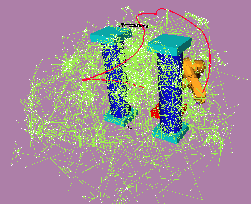
>>> EXERCISE 3: Run the PRM planner with the Gaussian sampling strategy to solve the TX90_R6_mobileBase demo.
Performance evaluation
Launch the benchmarking_PRM.xml already available at the Cube_Maze_R2 demo folder, to compare the basic PRM with different sampling strategies.
>>> EXERCISE 4: Analyze the results of the benchmarking, making emphasis on the time, the clearance and the number of graph states.
>>> EXERCISE 5: Repeat for different 2D environments (Cube-sPassage_R2 and Cube_Cluttered_R2).
>>> EXERCISE 6: Repeat for the TX90_R6_mobileBase demo.
RRT*
Open the demo demos/OMPL_geometric_demos/Cube_Maze_R2/OMPL_RRTStar_bigcube_maze2D_R2.xml to analyze how the RRT* planner solves the problem. The default parameter values of the demo will be used if not otherwise stated.
The Kautham interface to the RRT* planner has been designed to allow different optimization costs, length or clearance, according to the parameter Optimize dist(0)/clear(1), whose default value is 0. Here the default length optimization will be considered.
The rewiring process
To see how the RRT* keeps rewiring the nodes of the tree in order to optimize the solution path, the _MaxPlanningTime has been set to 1.0 (to let the generation of the first solution) and _Simplify Solution to 0 (not to allow the path simplification in order to better appreciate the changing of the solution). Now:
Set _Incremental to 1 and press Get Path to visualize the growing of the tree and its modification due to the rewiring process.
The topology of the solution can even change while optimizing its length, as it happen in the run shown in the video.
>>> EXERCISE 7: Repeat the process by setting the Range to 0.05.
>>> EXERCISE 8: Repeat for the TX90_R6_mobileBase demo. Is the initial path found able to be shortened? Which are the problems that RRT* faces for high-DOF problems?
Performance evaluation
Some of the parameters that modify the rewiring process are:
Rewire Factor: Scale factor used to control the number of neighbors considered in the rewiring process, i.e. the number of neighbors considered is the optimal number of neighbors multiplied by this rewiring scale factor.
Pruning (0/1): Parameter that controls whether the tree is pruned during the search. This pruning removes a vertex if and only if it and all its descendents passes a pruning condition (the pruning condition is whether the lower-bound estimate of a solution passing through the vertex is greater than the current solution).
>>> EXERCISE 9: Study the effect of these parameters and evaluate them using the benchmarking utility for the Cube_Maze_R2 problem.